<?xml version="1.0" encoding="utf-8"?><feed xmlns="http://www.w3.org/2005/Atom" ><generator uri="https://jekyllrb.com/" version="3.10.0">Jekyll</generator><link href="https://brookchuang1111.github.io/feed.xml" rel="self" type="application/atom+xml" /><link href="https://brookchuang1111.github.io/" rel="alternate" type="text/html" /><updated>2025-10-23T20:05:50+00:00</updated><id>https://brookchuang1111.github.io/feed.xml</id><title type="html">A Babbling Brook</title><subtitle>Hi I&apos;m Brook! I&apos;m majoring in data theory (math + stats) at UCLA. In my free time I like watching reality TV, acting as a matchmaker for my friends, and being a general menace.</subtitle><author><name>Brook Chuang</name></author><entry><title type="html">Chapter 3: Market Microstructure in Practice</title><link href="https://brookchuang1111.github.io/2025/04/24/ch3-mm.html" rel="alternate" type="text/html" title="Chapter 3: Market Microstructure in Practice" /><published>2025-04-24T00:00:00+00:00</published><updated>2025-04-24T00:00:00+00:00</updated><id>https://brookchuang1111.github.io/2025/04/24/ch3-mm</id><content type="html" xml:base="https://brookchuang1111.github.io/2025/04/24/ch3-mm.html"><![CDATA[<p>At last, here we are! The penultimate chapter of <em>Market Microstructure in Practice</em> by Lehalle and Laruelle focuses on optimal organization for optimal trading. We’ll look at fragmentation, market impact given the PFP, price anticipation and permanent market impact, price formation under conditioning, and orderbook dynamics.</p>

<p>Happy reading!</p>

<p>Below you can find a pdf of the textbook and my notes:</p>
<ul>
  <li><a href="/assets/market_micro/mm_textbook.pdf">Market Microstructure in Practice</a></li>
  <li><a href="/assets/market_micro/Ch_1_mm.pdf">Chapter 1 Notes</a></li>
  <li><a href="/assets/market_micro/Ch_2_mm.pdf">Chapter 2 Notes</a></li>
  <li><a href="/assets/market_micro/Ch_3_mm.pdf">Chapter 3 Notes</a></li>
</ul>

<h2 id="organizing-a-trading-structure-to-answer-a-fragmented-landscape">Organizing a Trading Structure to Answer a Fragmented Landscape</h2>
<p><strong>Main Inputs of Trading Tools</strong> <br />
Large asset managers concentrate on tasks of mounting and unwinding positions to dealing desks, which takes care of:</p>
<ul>
  <li>The relationships with intermediaries.</li>
  <li>Measuring trading costs and comparing broker performances thanks to Transaction Cost Analysis (TCA).</li>
  <li>Choosing benchmark to target (VWAP, TWAP, Implementation shortfall, Target Close) according to investment style that generated the trade.</li>
</ul>

<p>Dealing desks demand accuracy. Exchanges provide services around best execution (SOR), vendors provide better performance measurements and comparison features.</p>

<p><em>Market Data</em></p>
<ul>
  <li>Real time market data feeds are the eyes of a trading algorithm. Consolidated data is needed and the source should be easily disaggregated to know which trading venue is currently offering this price.</li>
</ul>

<p>Market data contains:</p>
<ul>
  <li>Market trades, described by price, quantity, and timestamp</li>
  <li>Limit orderbooks (bid-ask prices, quantities available, number of different market participants contributing at each price level), or sequences of modifications of the orderbook</li>
</ul>

<p>Data is enriched with analysis with bid-ask spread, qualifying the observed market trades, intraday volatility, efficient bid-ask spread, or estimates of hidden quantities in the book.</p>

<p><em>Connection to Venues</em> 
Algorithms need to be connected to exchanges. Connections are not natively synchronized with the market data and are two-way:</p>
<ul>
  <li>One to send messages to the trading venue: Creation of a new order, cancellation, or modification of another order.</li>
  <li>The other to receive messages from the trading venue about the orders of the trading algorithm. Acknowledgements of messages sent by the algo, rejections, cancellations, partial fills, ect.</li>
</ul>

<p>Incoming messages can be used as information probes. In dark pools, given no pre-trade transparency, orders sent by algos can be used as probes coming back with information about the state of the orderbook. When a dark buy order is filled at a given price, the orderbook of the dark pool contains resting sell quantities at the price or better.</p>

<p><em>Historical Data</em>
Optimal trading relies on intraday risk control and usual rhythms and behaviors of market features that are captured by models whose parameters are estimated by stock-by-stock or sector-by-sector basis. Historical data is needed and should contain:</p>
<ul>
  <li>Market Data (tick-by-tick or order-by-order)</li>
  <li>Analytics that have been computed in real time</li>
  <li>Recordings of the messages sent and received by the algorithms of the firm</li>
  <li>Context-related information lik news, corporate events, activation of circuit breakers, outages of trading venues, ect.</li>
</ul>

<p><em>Models</em>
A model is based off of three components:</p>
<ul>
  <li><em>The Formula</em>: Takes in input parameters and variables. Parameters can be estimated once per day and sorted, the variables are known in real time and have to be plugged in the formula on the fly.</li>
  <li><em>Estimation</em>: A mathematical procedure taking as input historical data on a given universe and a given horizon and computing estimated values of the parameters of the model.</li>
  <li><em>The accuracy computation</em>: A mathematical procedure to quantify the quality of the model and its parameters according to the immediate past or in real time.</li>
</ul>

<p><strong>Components of a Trading Algorithm</strong> <br /> 
Trading algos can be launched by a external user or by other algorithms. The different components are:</p>
<ul>
  <li><em>The execution parameters</em>: Defines the execution conditions that apply to the algorithm</li>
  <li><em>The risk control layer</em>: In charge of computing reasonable maximum and minimum trading rates to target during the trading: This is called the <em>trading curve</em>. The layer uses models and expected market contexts to produce minimum nd maximum trading envelopes to follow in order to make the balance between two main sources of risk: market impact and market risk.</li>
  <li><em>Trading robots or liquidity-seeking tactics</em>: Like SOR, these are more sophisticated opportunistic tactics dedicated to navigate inside the trading envelope defined by the risk control layer. These robots have to take into account the immediate state of the liquidity to extract as much value as possible from venues.</li>
</ul>

<p>The two layers, risk control and tactics, communicate through the risk control layer by sending messages to tactics to assign them short-term goals.</p>

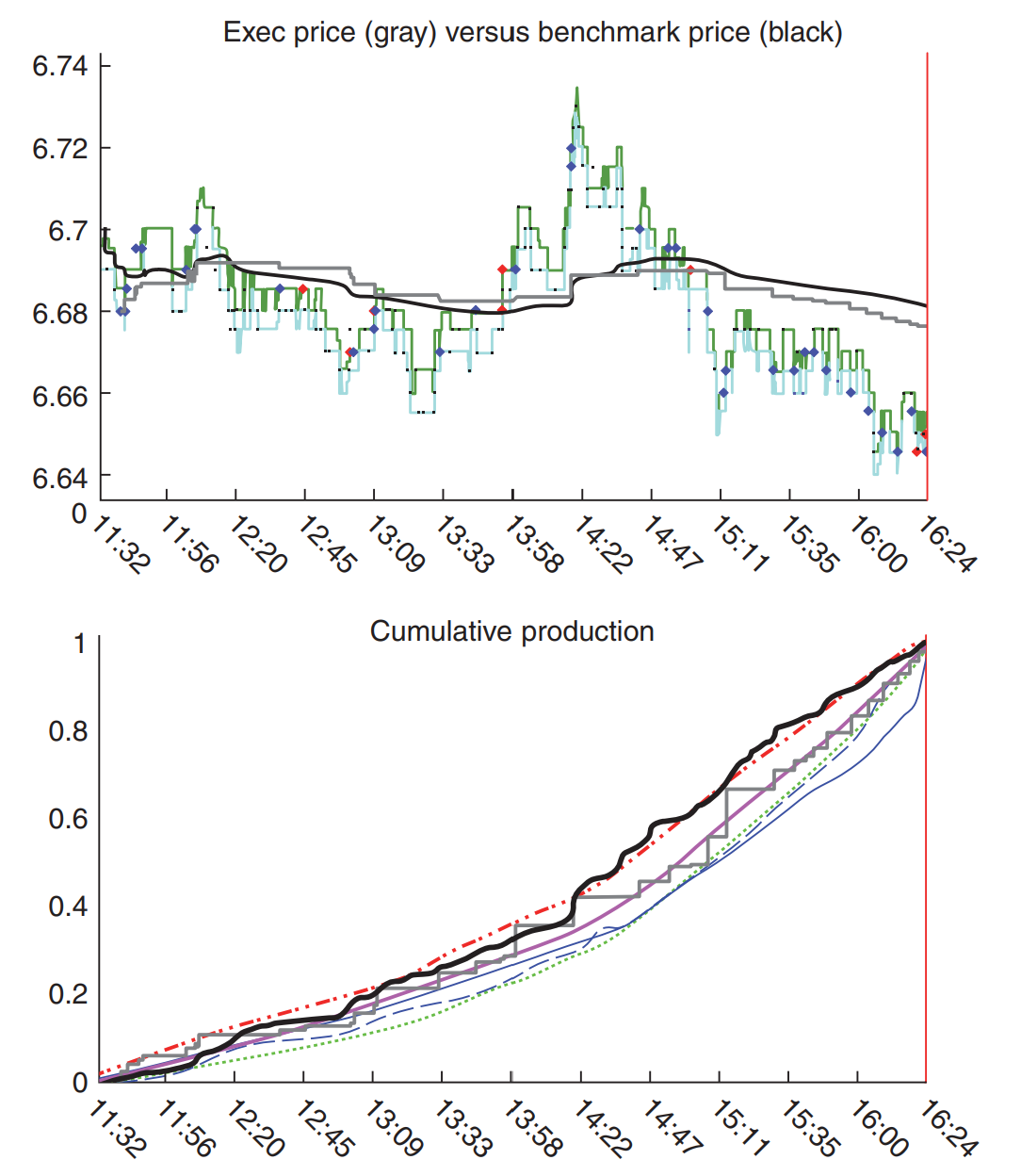
<p>In figure 1 the trajectory of a trading algo is shown with the trading envelope and the real trajectory of the algo.</p>

<!---Images-->
<figure style="display: flex; flex-direction: column; align-items: center;">
  <img src="/assets/ch3-mm/exec_price.png" alt="exec_price" width="400" />
  <figcaption>Figure 1. The price and the obtained trades (dots); below: The cumulated traded quantity by the algo (grey), by the market (dark), the envelope can be seen in dot-dash lines</figcaption>
</figure>

<h2 id="main-outputs-of-an-automated-trading-system-">Main Outputs of an Automated Trading System <br /></h2>
<p><em>Pre-trade Analytics</em>: The historical data, the models, and their parameters have to be used to provide decision support before the effective launch of a trading algorithm.</p>

<p>Pre-trade analytics are useful for the portfolios to check consistency of a portfolio and generate automated directives to speed up lines and slow down other according to pre-computation of the balance between expected market risk and expected market impact.</p>

<p>Typical pre-trade analysis includes:</p>
<ul>
  <li>Estimation and comparison of expected trading cost components (spread, traded volume, quantities on the books)</li>
  <li>Expected trading profiles</li>
  <li>Expected context (news, volatility levels)</li>
  <li>Breakdown by sector, currency, country, ect.</li>
</ul>

<p><strong>Monitoring Indicators</strong> <br />
Once an algo has been launched it has to be monitored by traders. Traders usually monitored several hundreds of working algos - indicators allow traders to build diagnoses of the algos on the fly.</p>

<p><strong>Performance Indicators</strong> <br />
A specific subset of monitoring indicators are direct measures of what the performance would be if trading should stop now and others include estimates of the performance when it will end, seen from now.</p>

<p>Typical performance indicators come from the decomposition of the average price of the trading algorithm according to different effects.</p>

<p>AVG price = Immediate Price + Market Moves + Market Impact.</p>

<p>On a benchmark-by-benchmark bases, such a decomposition can be refined towards</p>

<p>AVG Price = Immediate Price + Planned Price + Unexpected Market Moves + Trading Efficiency + Market Impact.</p>

<p><em>Planned price</em> is what the risk control part of the trading algo expected on average. <em>Trading efficiency</em> rates the success of the liquidity-seeking tactics used by the trading algo.</p>

<p><strong>Where to Produce Real Time Indicators</strong> <br />
Algorithms themselves produce the indicators to publish. <em>Indicator publishers</em> are compatible with the fact that trading algos can be modeled as stateless agents and should have introspection capabilities; publishing views on their own state in real time to share with final users of companion als is an important component of modern trading algos.</p>

<p><strong>Post Trade Analysis</strong> <br />
Three components should be compatible:</p>

<p>For the spread:</p>
<ul>
  <li>The pre-trade analysis gives an expected average value.</li>
  <li>The monitoring gives the current value, the updated expected average value, and the likelihood of the current value with respect to what happened so far. It gives the ability to quantify the relationship between the current trading performances and the trajectory of the spread.</li>
  <li>The post-trade analysis gives an assessment of the value of the spread during the trading and its influence on trading performance.</li>
</ul>

<p><strong>Transaction Cost Analysis (TCA)</strong> <br />
TCA is used by different algo providers to compare the efficiency of their trading over several weeks.</p>

<p>Post-trade analysis (day to day) aims to understand what happened because of the market context.</p>
<ul>
  <li>Requires fine grained analysis of market behavior.
TCA aims to to explain the part of performance comes from the design o the trading algorithms.</li>
  <li>Requires on averaging huge datasets to cancel most of market effects.</li>
</ul>

<p>TCA associates a given trading algo with a give market context of trading style so that the user of the algo will send flow to the proper algo provider given market conditions. TCA involves breakdowns according to the characteristics of the market (volatility, jumps, liquidity, occurrence of news, etc.).</p>

<p>Liquidity is important to consider given it is useless to compare the efficient of an execution on a very liquid stock with one illiquid stock.</p>

<p>Typical indicators used to quantify liquidity are:</p>
<ul>
  <li>bid-ask spread</li>
  <li>tick size in basis points</li>
  <li>quantity on the books</li>
  <li>daily turnover</li>
  <li>average trade size</li>
  <li>free float</li>
  <li>trading rate</li>
</ul>

<h2 id="market-impact-measurements-understanding-the-pfp-from-the-viewpoint-of-one-investor">Market Impact Measurements: Understanding the PFP from the Viewpoint of One Investor</h2>

<p>Factors that drive market impact:</p>
<ul>
  <li>liquidity of traded stock</li>
  <li>quantity which is executed relative tot he overall quantity traded by other participants</li>
  <li>aggressiveness of the trading algorithm</li>
  <li>duration of the execution</li>
</ul>

<p>Trade timing describes how an order is being traded compared to what happens in the market. Timing tells you if you are a trend follower or mean reverter. Timing tells you if the way you trade makes you visible to HFT eyes.</p>

<p><strong>Market Impact Over the Trading Period</strong> <br />
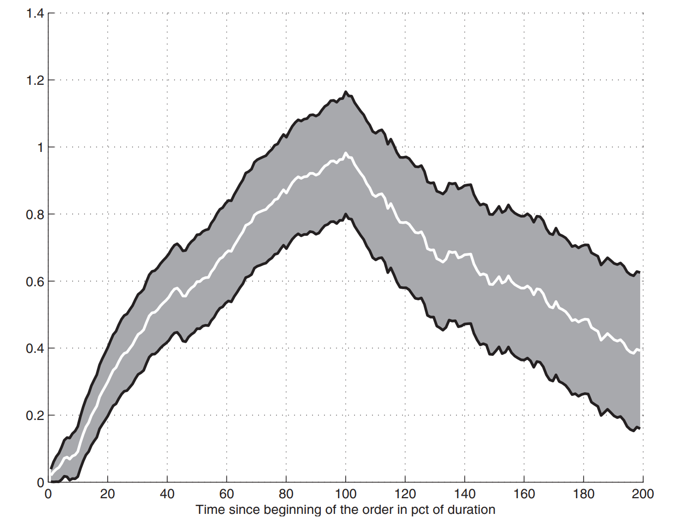
The benefit of intraday analysis of market impact is to quantify the <em>changes</em> in the market impact as an order is being executed and the <em>dilution</em> of this impact after the end of an execution.</p>

<p>The difference between the price at any given time and the arrival price is a good and frequently used measure of market impact.</p>

<!---Images-->
<figure style="display: flex; flex-direction: column; align-items: center;">
  <img src="/assets/ch3-mm/timing.png" alt="timing" width="500" />

  <figcaption>Figure 2. Intraday market impact in spreads</figcaption>
</figure>
<!---line break-->
<p><br /></p>

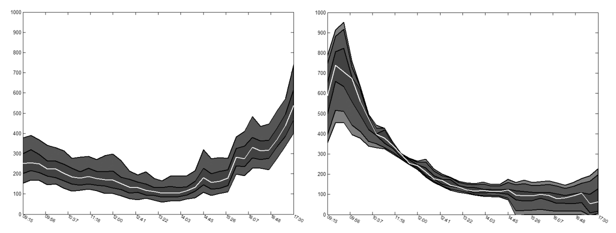
<p>Figure 2 shows the price of a stock while an order is being executed. If the returns of the stock is in the perspective of a buy order, prices above 0 means the investor will pay more to purchase a share or will be paid less to sell vs the beginning of execution. The grey bands represent the 95% confidence interval;the white line is the average. At 0 to 100 the impact curve is concave. At 100 to 200 shows the returns revert back.</p>

<p>Market impact may depend on several parameters.</p>

<p><em>Stock specific characteristics</em>:</p>
<ul>
  <li>liquidity of stock</li>
  <li>volatility</li>
  <li>spread size</li>
</ul>

<p><em>Order-specific characteristics</em>:</p>
<ul>
  <li>aggressiveness of execution</li>
  <li>quantity to execute</li>
  <li>expected duration</li>
</ul>

<p><strong>Structure of the Dependency Between Market Impact and Parameters</strong> <br />
<em>Period Liquidity Ratio</em> (PLR): participation rate</p>

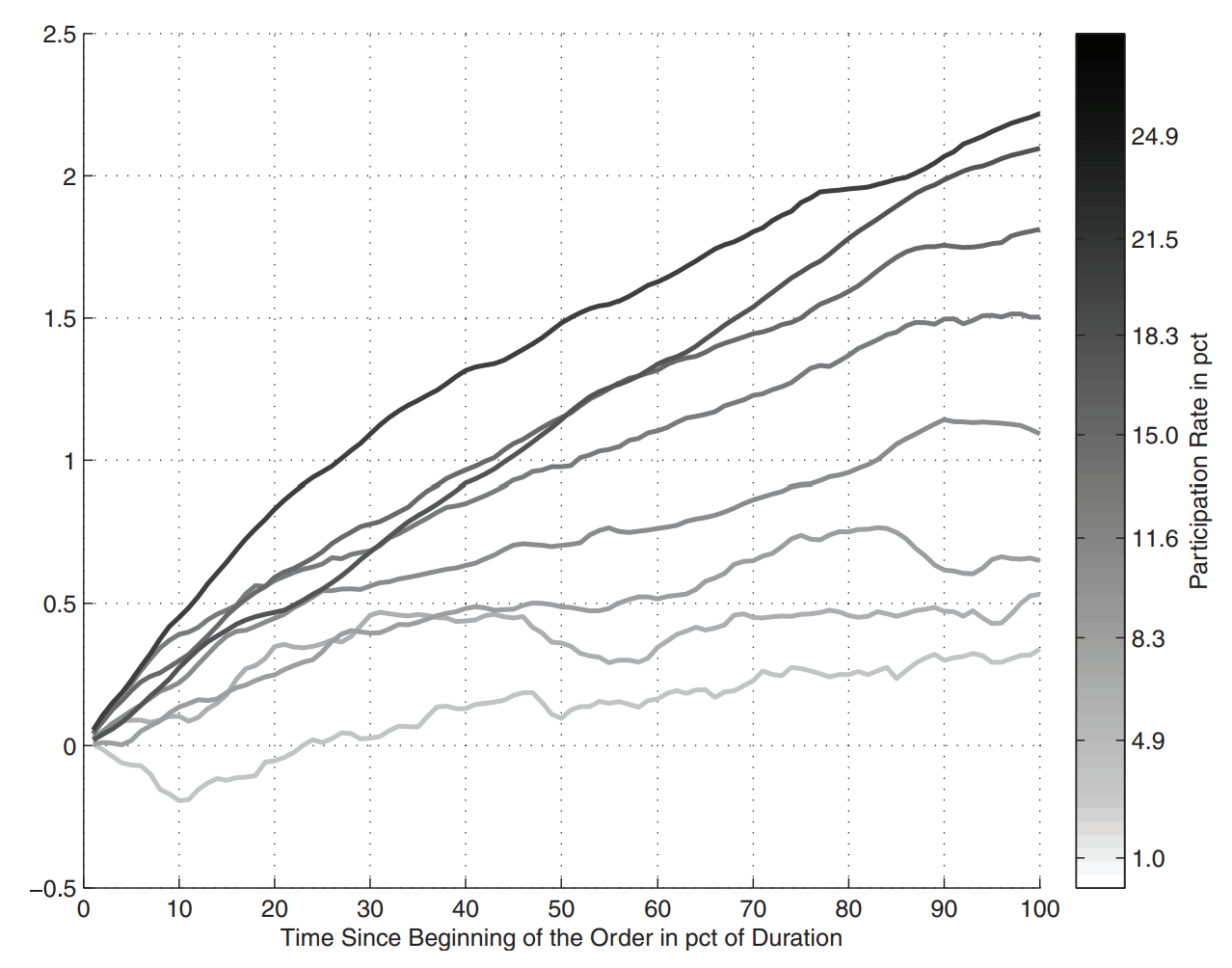
<p>In figure 3 we plot the market impact for different values of the participation rate. 
<!---Images--></p>
<figure style="display: flex; flex-direction: column; align-items: center;">
  <img src="/assets/ch3-mm/part_rate.png" alt="timing" width="500" />

  <figcaption>Figure 3. Intraday market impact in spreads depending on the participation rate</figcaption>
</figure>

<p>It can be seen that market impact curves get steeper as the participation rate increases.</p>

<!---Images-->
<figure style="display: flex; flex-direction: column; align-items: center;">
  <img src="/assets/ch3-mm/duration.png" alt="duration" width="500" />

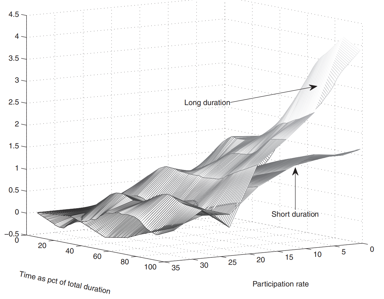
  <figcaption>Figure 4. Market impact vs. participation rate for two different sets of durations</figcaption>
</figure>

<p>In figure 4 we can see two impact surfaces for two different sets of durations. The surface corresponding to the long duration is always above the shorter duration - ie more market impact. Hence the longer the duration the bigger the impact.</p>

<p>With both participation rate and duration contributing to market impact, we can build the model:</p>

<!---Theorem box-->
<div style="border: 2px solid #ccc; border-radius: 8px; padding: 16px; margin: 20px 0; background-color: #f9f9f9;">
  <strong>Market Impact</strong>
  <p>
$$\begin{align}
\text{Market Impact } \propto \text{Duration}^\alpha \times \text{Participation}^\gamma
\end{align}$$
  </p>
</div>

<p>The dependency of the market impact on the two parameters separately is concave. This means the impact of one additional percent of participation rate for an order of a given duration is lower for higher participation vs lower participation.</p>

<p><strong>Market Impact on a Longer Horizon</strong> <br /> 
Within daily data the permanent market impact is the remaining price shift after the decay has taken place. The decay phase starts at the end of the execution period and can not be exactly determined - but we consider that the price reaches its final level after one day. Liquidity providers mostly react at the intraday timescale. After one day the temporary market impact of the metaorder execution vanishes.</p>

<p><strong>Price Anticipation or Permanent Market Impact</strong> <br /> 
There are two positions when it comes to permanent market impact.</p>

<p><em>Position 1</em>: Permanent impact as the consequence of a mechanical process.</p>
<ul>
  <li>Stock prices move because of the trading of all the market participants. If the selling pressure is stronger than the buying pressure, price goes down and vice versa if buying pressure is the strongest.</li>
  <li>We want to understand the law at the root of the impact of buying or selling pressure on price dynamics.</li>
</ul>

<p><em>Position 2</em>: Permanent impact as the trace of new information in the price.</p>
<ul>
  <li>Informational vision says stock prices move because new information is made available to market participants. New information allows investors to update expectations which leads to new global equilibriums and price levels.</li>
</ul>

<p><strong>Permanent Market Impact on a Long-term Horizon</strong> <br /></p>

<p>We will look at three studies that de-bias the effect of the signal that triggers price variations. This separates the information effect from the pure execution effect from permanent market impact.</p>

<p><em>[Bacry et al., 2015]</em>: Reports measures made on a database of electronically traded metaorders from the brokerage arm of a large European investment bank during 2010.</p>
<ul>
  <li>The broker execution database studied does not provide the informational content at the root of the trades.</li>
  <li>Authors assumed that the clients of the broker globally constitute a good representative sample of the diversity of market investors (total portfolio not far from CAPM)</li>
  <li>The study of price moves on the post-execution period net of market portfolio moves is the so called <em>idiosyncratic</em> moves of stock prices.</li>
</ul>

<p><em>[Waelbroeck and Gomes, 2015]</em>: Uses a database of trades from 112 portfolio managers across several large institutional asset managers between 2009 and 2012.</p>
<ul>
  <li>Each trade is labeled as ‘liquidity’ or ‘informed’ trades to separate trades triggered by informational events from the rest.
    <ul>
      <li>Informed: Metaorders coming from portfolio rebalancing.</li>
      <li>Uninformed: Cash trades that are related to new subscriptions of redemptions triggered by heterogeneous and relatively exogenous to the market information.</li>
    </ul>
  </li>
  <li>On a daily basis informed trades have a permanent market impact but uninformed trades do not.</li>
</ul>

<p><em>[Brokmann et al., 2015]</em>: Studies a proprietary CFM database consisting of an exhaustive list of 1.6 million metaorders together with the daily signals that lead to these trades over three full years (2011-2013) in a variety of equity markets.</p>
<ul>
  <li>Uses for each trade the signal that triggered it.</li>
  <li>Uses the intensity of the trading signal which triggered each metaorder to remove the informational content of their studied proprietary metaorder database.</li>
  <li>Divergence of effective and expected price moves gives measure of permanent impact in the absence of informational effect.</li>
  <li>Authors observed no permanent impact on the residual price moves.</li>
</ul>

<p><strong>De-biasing the Temporary Market IMpact of Autocorrelated Execution During th ePOst-Execution Period</strong> <br /></p>

<p>All three studies aggregate signed metaorder flows show autocorrelations even several days after execution. This has an effect of post-execution price variations and needs to be filtered out in order to make an accurate estimation of the permanent market impact.</p>

<p>Aggregated daily participation rates are computed at the stock scale as the sum of the signed traded volume divided by the total market volume for the stock on that day.</p>

<p>Total autocorrelations are the equi-weighted average of the autocorrelations across all the stocks of the studied universe.</p>

<p>Finding a unbiased long-term impact picture is not straightforward. Market impact of metaorders according to daily participation rate turns out to be far from linear.</p>

<p>Withdrawing impact of metaorders traded over the post-execution period uses a simple market impact model in [Waelbroeck and Gomes, 2015]. In  [Bacry et al., 2015] a square root model is fit. Price variations and the post-execution period are debiased by subtracting the market impact associated to the aggregated daily participation rate on that date applying the square root model.</p>

<p><strong>CAPM Decomposition of Price Variations</strong> <br />
[Bacry et al., 2015] uses a CAPM framework to disentangle the systematic component of the market impact form the idiosyncratic components. For each metaorder the decomposition is centered on teh execution dat over a 41-day period:</p>

\[\begin{align}
\forall d \in \{D-20, \dots, D, \dots +20\}, \\
\log(P_d) - \log(P_{d-1}) = \beta(\log(I_{d-1})) + \Delta W_d.
\end{align}\]

<p>$D$ is the metaorder execution date, $P_d$ is the stock’s close price on date $d$, $beta$ designates the beta of the traded stock on the period from $D-20$ to $D+20$, and $I_d$ is the reference index price on date $d$.</p>

<p>$\beta$ is estimated through simple least mean square regression and the idiosyncratic component starting one day before the execution at date $D-1$ is defined as the cumulative sum of the residuals $\Delta W_d$:</p>

\[\begin{align}
W_d - W_{D-1} = \sum^d_{d=D}\Delta W_k
\end{align}.\]

<p>The systematic component is defined as $\beta(\log(I_{d-1}) - \log(I_{D-1}))$.</p>

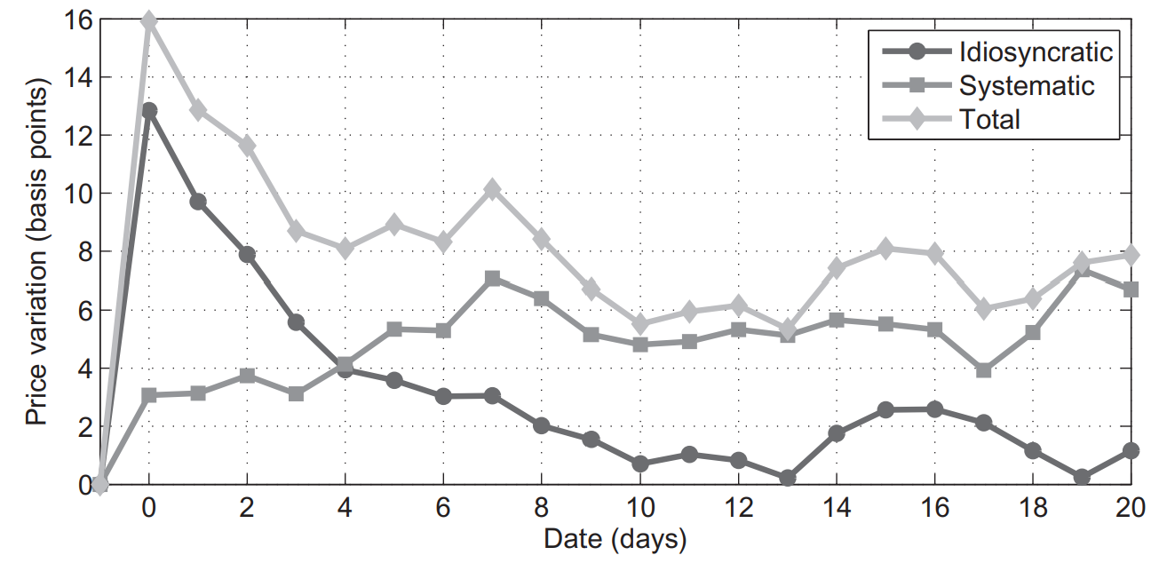
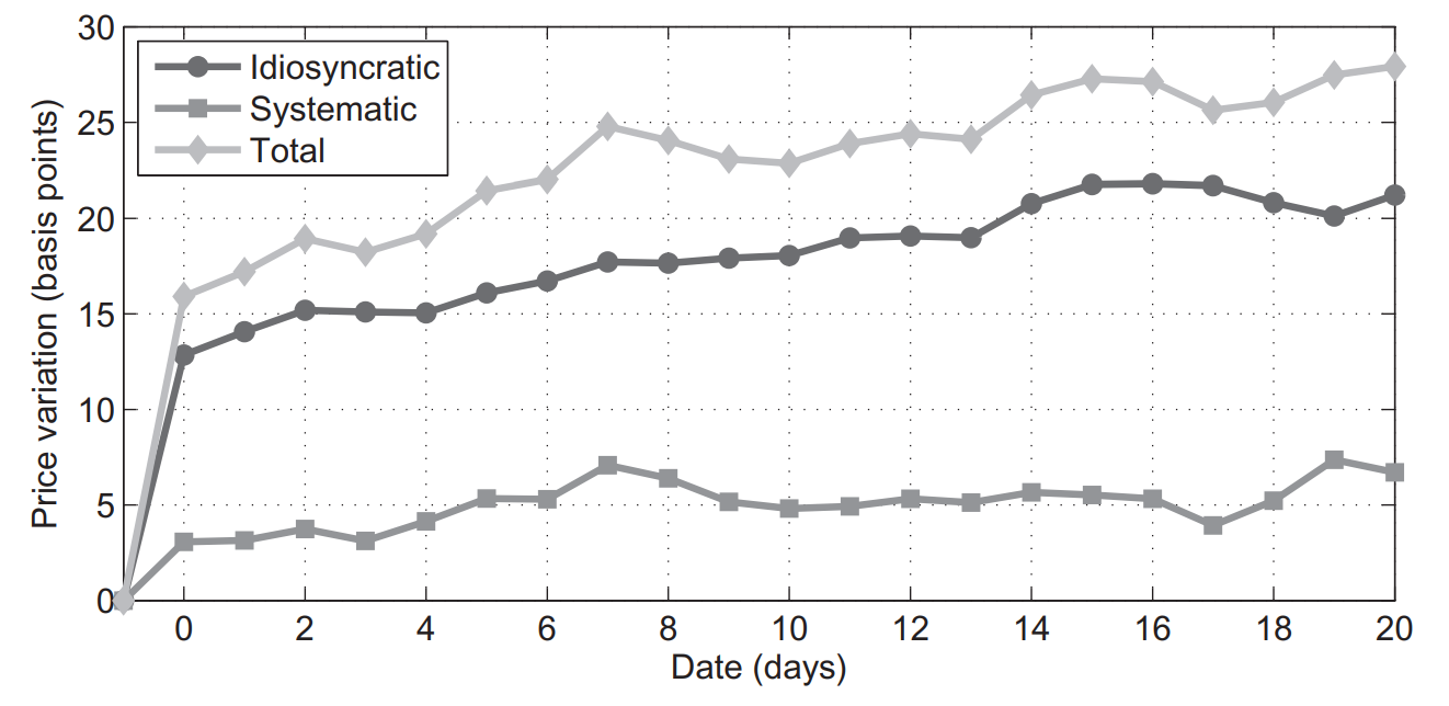
<p>In figure 5 we see the idiosyncratic, systematic, and daily post-execution profiles of price moves. The post-execution profiles of price moves are not yet debiased - the price jump between day 0 and 1 correspond to the market impact of the execution on day 1. Over the time horizon prices slowly trend in the same direction. 
<!---Images--></p>
<figure style="display: flex; flex-direction: column; align-items: center;">
  <img src="/assets/ch3-mm/idio.png" alt="idio" width="500" />

  <figcaption>Figure 5. Post-execution profile relative to close price on the day before
execution. Idiosyncratic component + systematic component = total component</figcaption>
</figure>

<p>After debiasing the post-execution profile the market impact of metaorders executed the day after the execution has been removed. We can see the effect in figure 6.</p>

<!---Images-->
<figure style="display: flex; flex-direction: column; align-items: center;">
  <img src="/assets/ch3-mm/idio_debiased.png" alt="idio_debiased" width="500" />

  <figcaption>Figure 6.  Post-execution profile without the impact of other metaorders. Price moves are considered relatively to close price the day before execution. Idiosyncratic component + systematic component = total component</figcaption>
</figure>

<p>Over the post-execution period the price converges back to a level lower than the one reached on execution day. The idiosyncratic post-execution profile reaches its initial level before the end of the observed period - this permanent market impact that remains 20 days after the execution is entirely explained by the systematic component (average level of the market).</p>

<p>Based on this, [Bacry et al., 2015] concludes that once temporary market impact of the correlated metaorders executed has been removed and aggregated information (systematic) has been isolated and removed there is no permanent market impact due to the metaorder itself.</p>

<h2 id="the-pfp-and-orderbooks-dynamics">The PFP and Orderbooks Dynamics</h2>
<p>On equity markets most trading takes place on LOB that are often called CLOB. This is opposite of a quote driven system (used on fixed income markets).</p>

<p><strong>Attractiveness of Limit Orderbooks</strong> <br /> 
Limit orderbooks are convenient for several reasons:</p>
<ul>
  <li>They are anonymous and provide MLT, leveling the playing field between traders and market-makers.</li>
  <li>They are fast and synchronized, easily supporting fragmentation and competition between trading platforms.</li>
</ul>

<p>By understanding orderbook dynamics one can answer the question: <em>How can practitioners extract information form orderbook dynamics?</em></p>

<p><strong>Information Reaching Orderbooks</strong> <br />
At the start of the day an orderbook is empty. Traders and market makers send orders that are stored in the orderbook if they do not match resting orders - orders are matched if they are compatible in price. Each match generates a transaction and gives birth to three messages:</p>
<ul>
  <li>Public trade</li>
  <li>Two private trades: one for each party of the trade</li>
</ul>

<p>Because the orderbook is hosted on a server in a data center, the localization of the data center is paramount because it influences latency.</p>

<p>Members of the trading facility are connected to the server ina secured way, often via tow channels: one private (SLE) allowing them to send and receive messages to the server and one public channel (SLC).</p>
<ul>
  <li>On the private connection the trader will send specific order to the matching engine and receive answers and messages concerning his orders.</li>
  <li>On the public channel they will see the transactions and the state of the orderbook.</li>
</ul>

<p><strong>The Orderbook in Motion</strong> <br /> 
If the fair price of a stock is around $10, the first trader with intentions to buy will buy cheaper and a selling trader will try to sell for more. This message of buying low and selling high can last long as no transaction occurs. It shapes the orderbook and keeps record (limit-by-limit view) of the sum of all orders at each level of price.</p>

<p>To see the trade the order must be fulfilled. At any point in the life cycle of the orderbook a trader can insert, modify, or cancel an order.</p>

<p>The effect of messages can:</p>
<ul>
  <li>Remove liquidity via cancellation or transaction (Market order or limit marketable order).</li>
  <li>Add liquidity via an insertion.</li>
</ul>

<p>Transactions can only occur at the first limits of the LOB.</p>

<p><strong>Understanding via Conditioning</strong> <br /> 
To use conditioning of the orderbook we focus on the probability  that a limit order touches the first limit only when its size is large. Is the probability different from the probability of an insert at the second limit when it is small?</p>

<p>This conditioning can be split into three trends:</p>
<ul>
  <li><em>Zero-intelligence</em>: Has few conditioning and instead focuses on identifying the distribution of variables of interest.</li>
  <li><em>Game theoretic</em>: Explains the behavior of participants with accuracy. Tries to deduce the theoretical laws for probability of each type of order.</li>
  <li><em>Empirical</em>: Authors estimate transitions empirically.</li>
</ul>

<p><strong>Poisson Modeling</strong> <br />
We can use the point process to model the probability of occurrence of an event. Poisson processes are standard point processes with intensity $\lambda$. Let $N$ be the number of occurrences of an event, then we can same for some time $t$:</p>

\[\begin{align}
\lambda = \lim_{\Delta t \to 0}\frac{\mathbb{E}(\Delta N)}{\Delta t}. 
\end{align}\]

<p>If we know $\lambda$ then the average number of events observed during $\Delta T$ can be approximated using $\lambda \times \Delta T$.</p>

<p>Hence we can isolate three intensities in the orderbook:</p>
<ul>
  <li>$\lambda^+$: limit order</li>
  <li>$\lambda^c$: cancellation</li>
  <li>$\lambda^x$: transaction</li>
</ul>

<p><strong>Plain Homogenous Poisson Modeling</strong> <br /> 
The simplest model for the three intensities is to use the <em>homogenous Poisson framework</em>. The probability to observe a liquidity consuming or liquidity providing event is independent of the state of the orderbook.</p>

<p>We can estimate the intensities by starting at time $t$ and record the timestamps of the next event in each category, which we denote $\tau^+, \tau^c, \tau^x$. Obtain the observations of time to wait $\tau - t$ then average them out over the whole database for an estimate of $1/\lambda$.</p>

<p>With the three intensities we can simply run a simulation of the random dynamics of an orderbook and look at the distributions of the queue sizes we obtain during the simulation.</p>

<p>The homogenous Poisson process is very far away from reality. It does not take into account the state of the orderbook. <em>Modeling arrival rate of atomic events (insert, trade, cancel) does not succeed in recovering the observed configurations of queue sizes on the same data</em>.</p>

<p><strong>Improving the Model Based on Conditioning</strong> <br /> 
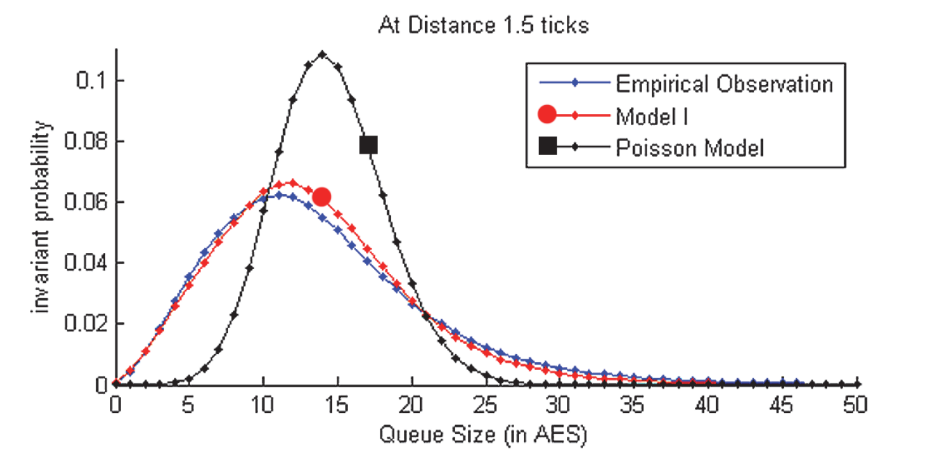
[Huang et al., 2015] shows a good way to improve the modeling by simply conditioning the three intensities by the size of the considered queue. This is called the <em>Queue Reactive Model</em>.</p>

<p><em>Model I</em>
Instead of avenging the time before events to find the intensity, we keep record of one intensity for each queue size:</p>
<ol>
  <li>Start at time $t$.</li>
  <li>Record the queue size $Q_t$ at $t$ in a generic unit.</li>
  <li>Observe an event (say $c$) at $\tau^c$.</li>
  <li>Keep track of $\tau^c - t$ in a register associated to the size of the queue $Q_t^c$ at $t$.</li>
</ol>

<p>Iterating over a lot of starting times $t$ gives us a collection of $\tau - t$ for each event. We can now average wait times by queue size.</p>

<!---Images-->
<figure style="display: flex; flex-direction: column; align-items: center;">
  <img src="/assets/ch3-mm/poiss.png" alt="poiss" width="500" />

  <figcaption>Figure 7.  Asymptotic distribution of the size of the second queue in three cases:
Empirical and “Model I” of [Huang et al., 2015] are very close, the Poisson model
(upper dark line), is very different. x-axis is observed queue size in AES, y-axis is
the probability of occurrence of this size</figcaption>
</figure>

<p><em>Model II \&amp; III</em> 
The distribution of sizes at other limits are not good with Model I, so Model II and III improve the statistics by conditioning intensities by the current size of other queues.</p>

<p>These models condition intensities by the size of the concerned queue but also by the size of its two neighbors. For example the intensity of events ont he first queue should be a function of the current size of the first, the second, adn the opposite first queue. To predict probability $p$ of the number of cancellations int he next 10 seconds on the first bid queue of size 4, we can write:</p>

\[\begin{align}
p := \lambda^c(4, 2, 1) \times 10.
\end{align}\]

<p>The improvement can be describes by two facts:</p>
<ul>
  <li>When the first queue is smaller than its opposite queue, it will most probably be consumed.</li>
  <li>When a first queue is large, the second queue will probably see more cancellations than if the first queue is small.</li>
</ul>

<p>This is called <em>predictive power of imbalance</em>: liquidity imbalance at the first limit gives a god idea of future price direction.</p>

<p>In most cases the amplitude of this future price movement is lower than a tick size, hence it is not possible to build a rewarding arbitrage on this predictor.</p>

<p><strong>Asymptotic Behaviors of the First Two Queues</strong> <br /> 
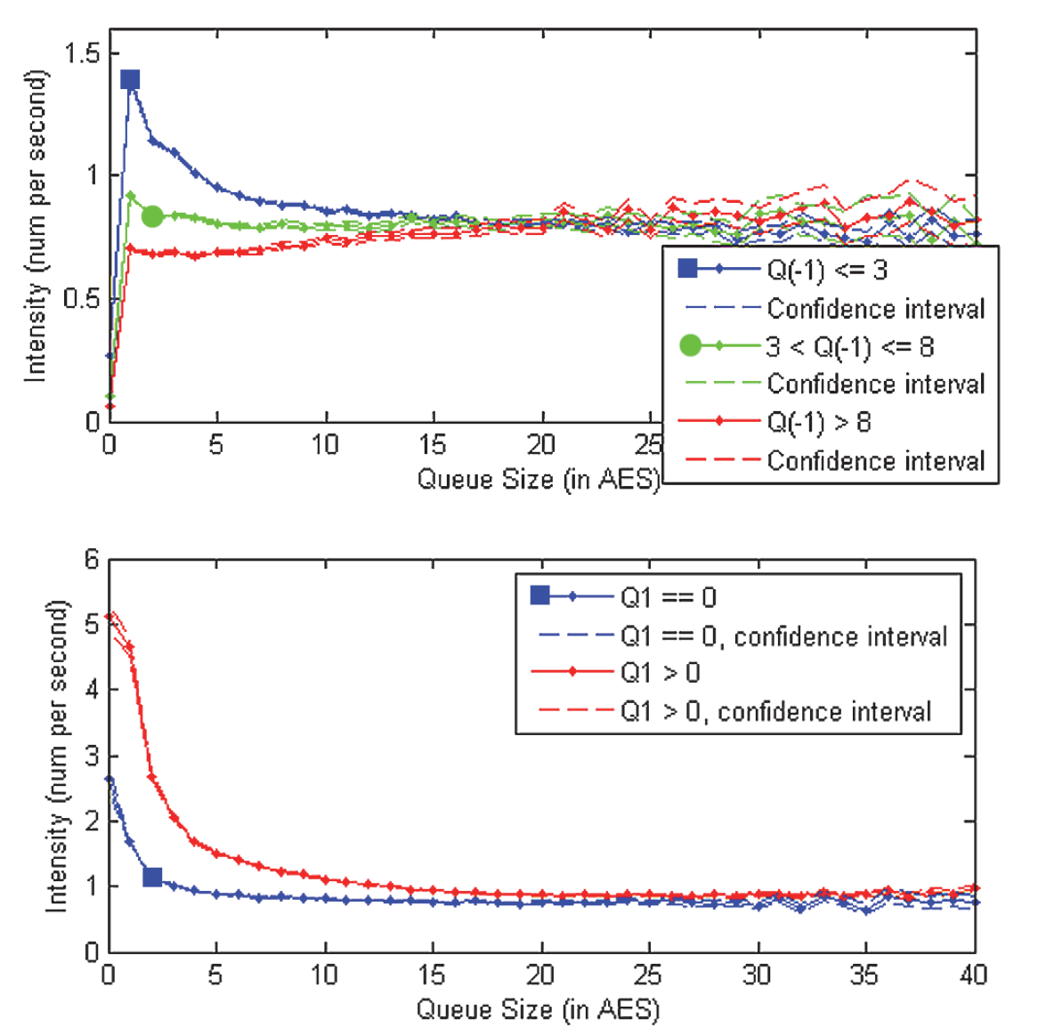
<em>A/R ratio</em> (Arrival over Departure ratio): This measures the intensity of insertion over te sum of the intensities of cancellation and trades.</p>

<p>When the ratio is greater thn one,the queue will explode (size will never stop increasing) and when its ratio is lower than one the queue will disappear (size will go to zero).</p>

<!---Images-->
<figure style="display: flex; flex-direction: column; align-items: center;">
  <img src="/assets/ch3-mm/ar.png" alt="ar" width="500" />

  <figcaption>Figure 8. Ratio of incoming over outgoing liquidity on first limit (top) and
second limit (bottom) as a function of its size (x-axes)</figcaption>
</figure>

<p>In figure 8 we can see</p>
<ul>
  <li>The first limit is always depleting to 0.</li>
  <li>The second limit explodes.</li>
</ul>

<p>In the context of stable sizes of the orderbook:</p>
<ul>
  <li>The first queue goes to 0 while the second queue explodes.</li>
  <li>Once the first queue disappears the formerly second queue is now promoted as a first queue.</li>
  <li>The promoted queue depletes to prevent explosion.</li>
</ul>

<p><strong>Liquidity Dynamics vs. Price Dynamics</strong> <br /></p>

<p>Note an observation: Now that we have a model reproducing with accuracy liquidity dynamics, you can generate realistic orderbook dynamics - <em>but what about price trajectories you generated?</em></p>

<p>The volatility of these trajectories is far too low compared to the ones observed in the real database used to fit the intensities. This is because in the simulations where a queue is promoted, the sizing of the new first queue is very large. This leads to <em>price reversion</em> - the negative autocorrelation of intraday price returns is a well-known stylized fact, but for an orderbook driven mode, the effect is too strong.</p>

<p>To compensate for the mean reversion we can introduce the following mechanisms:</p>
<ul>
  <li>Time to time: when a first queue fully depletes.</li>
  <li>All market participants accept the newly set price as a new ‘fair price: as a consequence the model has to reset the orderbook state to a randomly chosen one in the database.</li>
</ul>

<p><strong>Summary</strong> <br />
The Queue Reactive Model of orderbook dynamics shows the following:</p>
<ul>
  <li>Predictive power of the imbalance of provided liquidity (sizes of first two limits)</li>
  <li>The usefulness of the heterogenous Poisson process to roughly model the occurrence of orderbook events.</li>
  <li>The need to condition the intensity of the arrival rates of such events byt he size of the concerned queue (and its neighbors).</li>
  <li>The need to add a reset of orderbook state after price movement to prevent intense price mean reversion.</li>
</ul>

<p>When tick size is large the liquidity contained in each queue will be more meaningful than when the tick is small.</p>

<p>The point process in the orderbook is important but other models exist. Instead of counting instance in time, we can count events - changing the meaning of the obtained models. These are called propagator models.</p>

<h2 id="optimal-trading-methods">Optimal Trading Methods</h2>

<p><strong>Algorithmic trading: Adapting Trading Style to Investor Needs</strong> <br /> 
The following can be noted in electronic execution from investors:</p>
<ul>
  <li>In the US, HFTs are almost everywhere - stealth trading is the main point of focus.</li>
  <li>In Asia the comparison between the efficient of trading in each local market is very importance.</li>
  <li>In Europe the need to mix between avoiding being detected by HFTs and understanding the efficient of interacting with a set of orderbooks to adjust order routing policies as fast as possible.</li>
</ul>

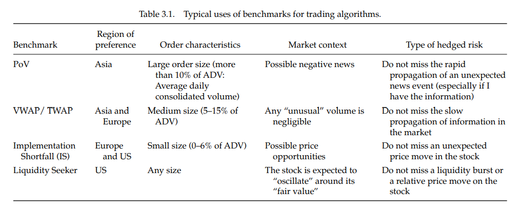
<p>European investors should target Implemented Shortfall benchmarks, Asian ones should focus on VWAP or PoV, and US ones  should look at liquidity seekers.</p>

<p>Liquidity seekers are more suitable to trading orders without minimum participation rate constrains, IS are for small orders, VWAP are for larger ones and PoV for very large ones.</p>

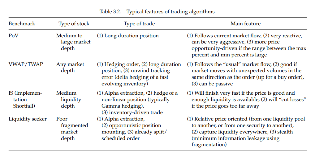
<p>The textbook summarizes stock features and features of trading algos in the tables below:</p>

<!---Images-->
<figure style="display: flex; flex-direction: column; align-items: center;">
  <img src="/assets/ch3-mm/t1.png" alt="t1" width="700" />

  <figcaption>Figure 9.</figcaption>
</figure>

<!---Images-->
<figure style="display: flex; flex-direction: column; align-items: center;">
  <img src="/assets/ch3-mm/t2.png" alt="t2" width="700" />

  <figcaption>Figure 10.</figcaption>
</figure>

<p><strong>Customization Offers Multi-feature Trading Styles</strong> <br /> 
These benchmarks can be combined: we can add maximum and minimum participation rates to an algo to make it behave like a PoV in the case of a really high or low market volume during the trading.</p>

<p>You can match sophisticated benchmarks like ‘follow market flows if there is high volume, finish fast if the price is really low, and use as much liquidity as possible’ using VWAP or TWAP as a backbone with a minimum participation rate.</p>

<p>Market data needed to build benchmark based policy are noisy because of HFT activity in the orderbook and uncertainty on some important parameters.</p>

<p>From a practical standpoint the optimal trading curve o follow is expressed as a trade rate that has to be represented by the algorithm. If it obtains trades too fast with respect to this curve, it has to stop posting; if it does not obtain enough it needs to obtain trades more aggressively, paying the spread. The curve is not a thin line but a thick one (given noisy data) such that it can define a <em>trading envelope</em>. Inside the envelope any trading trajectory cannot a priori be said to be more efficient than another from a risk-control perspective.</p>

<!---Images-->
<figure style="display: flex; flex-direction: column; align-items: center;">
  <img src="/assets/ch3-mm/enve.png" alt="enve" width="700" />

  <figcaption>Figure 11. Trading envelopes at different risk levels for a VWAP (left) or a (right)
trading algorithm</figcaption>
</figure>
<p>Inside a trading envelope any combination of liquidity capturing techniques can be plugged in without harming the optimality of the risk control layer (strategic layer). It is also possible to inject any volume or price-driven constraints if needed into the way they are built. Customization of a trading algo follows a two step process:</p>
<ol>
  <li>Understanding the desired risk profile and injecting the needed constraints into the trading envelope building process</li>
  <li>Understanding the mix of liquidity adapted to the investment style and plugging the associated tactics into the envelopes with respect to properly defined market conditions.</li>
</ol>

<p><strong>Liquidity Seeking Algorithms are no Longer Nice to Have</strong> <br />
Any market participant should be able to evenly access all of the trading venue quoting a given instrument. Any investor should be able to access all the available liquidity at a given marketable price.</p>

<p>In the US the <em>trade-through rule</em> demands that trading venues themselves reroute orders that are marketable at a better price elsewhere. In Europe, the executing broker is in charge of the kind of rerouting - they have to disclose to their clients the <em>best execution policy</em> explaining his rerouting methodology.</p>

<p>The difference is important:</p>
<ul>
  <li>In the US the trading venues have to be able to access an official consolidated orderbook. The clearing and settlement fees/costs have to be the same for all trading venues otherwise a market participant could direct a marketable order on a venue that seems to offer a cheaper price than another (but the participant will pay more, all costs included).</li>
  <li>In Europe the executing brokers are in charge to select the way they offer consolidated access to liquidity and have to prove it. It increases the cost of fragmentation for the intermediaries and demands that the investors are able to understand the stakes of these ‘consolidated services’.</li>
</ul>

<p><strong>Impact of Trading Costs/Fees</strong> <br /> 
Let us denote venue $V$ at price $P$ with fees $f$. Is it cheaper to remove liquidity on another venue $V’$ at a higher price (for a buy order) $P(1+\delta)$, where $P\delta$ is the tick size in euro, because of cheaper fees (say the fees on $V’$ are $f’$ and on $V$ they are $f$ such that $f’ = f - \phi$).</p>

<p>If we have a better price on venue $V’$ than on $V$ we can write:
\(\begin{align}
P(1+\delta)(1+f-\phi)Q &lt;P(1+f)Q.
\end{align}\)</p>

<p>This is equivalent to having the tick size (in basis points) small enough such that:</p>

\[\begin{align}
\delta &lt; (1 - \frac{\psi}{1+f})^{-1} - 1 \approx \phi.
\end{align}\]

<p>This means that the tick size should be as small as the fee difference.</p>

<p>A liquidity provider has to be sensitive to the fees he or she will have to pay once this order will be executed. Most times an observer can expect to see limit orders going first on the cheapest venue.</p>

<p><strong>Impact of Latency</strong> <br /> 
It can be said that what is important is not the liquidity that can be seen in the orderbooks but the <em>probability that you will be able to obtain liquidity at a given price level when your order reaches the orderbooks</em>, taking into account the latency discrepancies between venues, the mirrored orders, and hidden liquidity.</p>

<p><strong>Seeking an Optimal Liquidity Capturing Scheme</strong> <br /> 
Dealing with a marketable order (buy market order or buy order with a limit price higher than the best ask price on at least one trading venue) has shown that effects to take into account are as follows:</p>
<ul>
  <li>Probability of hidden liquidity in the orderbooks.</li>
  <li>The probability that when the latency to all venues is not the same, HFTs take advantage of information conveyed by market orders reaching one venue to cancel their liquidity providing orders.</li>
</ul>

<p><strong>Building a Liquidity Seeker</strong> <br />
A liquidity seeker has to take care of the following:</p>
<ul>
  <li>Removing liquidity optimally using estimates of the hidden liquidity, mirrored orders, and latency to each venue open to trading.</li>
  <li>Posting limit orders optimally to end an order as fast as possible.</li>
</ul>

<p>Like in dark pools, liquidity in any pool is clustered. Once a trade has occurred, the probability of observing another one increases.</p>

<p>Using fill rates and real liquidity estimates, we can find the optimized allocation of quantity to trade across different trading venues.</p>

<hr />
<p>Well, this is the end of my mini series! Don’t fret, I have more microstructure posts coming soon; specifically look out for some analysis on the papers mentioned in the textbook.</p>

<p>But anyways, I hope you enjoyed my aggregated notes, both transcribed and hand written, and that you learned something cool.</p>

<p>As a reward for staying till the end, here’s a picture of Linnea’s cat:</p>

<!---Images-->
<figure style="display: flex; flex-direction: column; align-items: center;">
  <img src="/assets/ch3-mm/cat.jpeg" alt="enve" width="400" />
</figure>]]></content><author><name>Brook Chuang</name></author><category term="Market Microstructure" /><summary type="html"><![CDATA[At last, here we are! The penultimate chapter of Market Microstructure in Practice by Lehalle and Laruelle focuses on optimal organization for optimal trading. We’ll look at fragmentation, market impact given the PFP, price anticipation and permanent market impact, price formation under conditioning, and orderbook dynamics.]]></summary></entry><entry><title type="html">Chapter 2: Market Microstructure in Practice</title><link href="https://brookchuang1111.github.io/2025/04/21/ch2-mm.html" rel="alternate" type="text/html" title="Chapter 2: Market Microstructure in Practice" /><published>2025-04-21T00:00:00+00:00</published><updated>2025-04-21T00:00:00+00:00</updated><id>https://brookchuang1111.github.io/2025/04/21/ch2-mm</id><content type="html" xml:base="https://brookchuang1111.github.io/2025/04/21/ch2-mm.html"><![CDATA[<p>In Chapter 2 of <em>Market Microstructure in Practice</em> by Lehalle and Laruelle we explore the nuances of fragmentation by looking at volume curves, the four main variables of liquidity, market share’s effects on spread, and the agenda of HFTs.</p>

<p>I’ve omitted most of the appendix material, historical analysis of European alternative markets, and the Spanish Experiment. For the curious reader more details can be found in Chapter 2.5.</p>

<p>This post is a continuation of Chapter 1, which can be found under ‘Market Microstructure’ on my ‘Blog Posts’ tab. Happy reading!</p>

<p>Below you can find a pdf of the textbook and my notes:</p>
<ul>
  <li><a href="/assets/market_micro/mm_textbook.pdf">Market Microstructure in Practice</a></li>
  <li><a href="/assets/market_micro/Ch_1_mm.pdf">Chapter 1 Notes</a></li>
  <li><a href="/assets/market_micro/Ch_2_mm.pdf">Chapter 2 Notes</a></li>
  <li><a href="/assets/market_micro/Ch_3_mm.pdf">Chapter 3 Notes</a></li>
</ul>

<h2 id="intraday-market-share-to-volume-curves-stationary-issues">Intraday Market Share to Volume Curves: Stationary Issues</h2>
<p>Not all market participants trade for the same reasons. Hence, when liquidity providers create bridges among pools of liquidity, liquidity remains concentrated.</p>

<p>To catch the reference price, primary markets are preferred because they create these reference prices.</p>

<p>Primary markets maintain a monopoly on the flow of another reference price effect called the <em>Exchange Delivery Settlement Price</em> (EDSP). This is the reference price that will be used for the valuation of the derivatives at the expiry.</p>

<p><strong>Inventory Driven Investors Need Fixing Auctions</strong><br />
Equity trading consists of two types of trading sequences:</p>
<ul>
  <li><em>Continuous phase</em>: This consists of immediate trade execution where both sides of the orderbook match.</li>
  <li><em>Fixing Auction phase</em>: this phase includes both opening and closing auctions that are important to fill and clear the orderbook. One can have up to four auctions at once. Some exchanges omit the continuous phase.</li>
</ul>

<p>Fixing auctions are used for consensual pricing and to unwind orders with huge volume. During witching days fixing turnover is high given that derivative products that expire are taken or closed during these auctions to benefit form same price.</p>

<p>By concentrating more agents, fixing auctions are allowed to form a more consensual price for the whole volume traded. This is very useful if the price is a reference for many valuations (closing prices usually are) and to build orderbooks before the opening of the market.</p>

<p>Fixing auctions also reduce price impact of a trade given high volatility - enhancement of info revealed during the auction stabilizes volatility and increases price stability.</p>

<p><strong>Rules of Call Auctions</strong><br />
Fixing price is determined by four steps - if the price is not clear by the first step the next step is applied. If the last step is not applicable the fixing price can not be determined.</p>
<ol>
  <li><em>Maximum Executable Volume</em>: Establish the price at which the highest quantity will be executed.</li>
  <li><em>Minimum Surplus</em>: Determine price based on the minimum quantity left in the market at the fixing price.</li>
  <li><em>Market Pressure</em>: If surplus is wholly on the buy side then the highest potential price is the fixing price. Vice versa is true. If surplus is on both sides then the next rule is applied.</li>
  <li><em>Reference Price</em>: The reference price is the last price traded.</li>
</ol>

<p>Different methodologies exist for different exchanges.</p>

<p><strong>Theoretical Matching Curves</strong><br />
The composition of participants is different with opening and closing auctions.</p>

<p><em>Matching Curves</em>: Relative difference between the volume that would be matched at time $t$ if the auctions ended at time $t$ with the final volume matched at the real fixing for each time $t$.</p>

<p>When a matching curve is zero this means total end volume has been sent to the market - every participant revealed its desire to trade.</p>

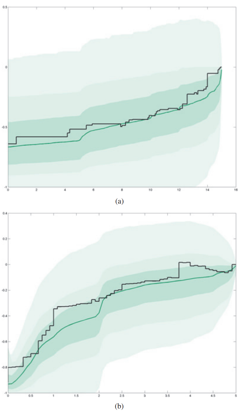
<p>In the pre-opening period book building accelerates as time goes on. Matched volume only reaches its final volume in the last few moments. The curve is convex in figure 1.</p>

<p>During closing call, matched volume rapidly increases to its final level as agents already present must participate in the fixing order to close positions. The curve is concave.</p>

<p>Participants take longer to intervene in opening vs closing because there is less uncertainty but also less patience at the end of the day. Participants face most constraints in the closing session given its the last time to open or close a position for the day.</p>

<!---Images-->
<figure style="display: flex; flex-direction: column; align-items: center;">
  <img src="/assets/ch2_mm/matching_cruve.png" alt="curve" width="300" />
  <figcaption>Figure 1. Matching curves (convergence of theoretical fixing volume to its final value) with the inter-quartile range (grey) and a sample day (black) for Crédit Agricole during opening auctions (a) and closing auctions (b) </figcaption>
</figure>

<p><strong>The Opaque German Orderbook</strong> <br />
For closing call matching curves in other markets, more than 90% of the distribution remains below the final value. This means that 50% of the time the final volume will be reached before the end of th fixing auction. The upper quartile will go higher than the zero threshold - and given our fixing pricing rules of maximizing volume - this means that a certain amounts of orders needed to be cancelled or modified before the end (around 25%).</p>

<p>In German auctions the orderbook is not revealed. The orders cancelled are probably players fishing for information by cancelling and sending orders to test fill rates. Exploitation/exploration tradeoffs are needed to optimize information levels in the orderbook.</p>

<p><strong>Information Peaks</strong> <br /> 
The pace of information sent into closing and opening auctions follow certain patterns. These updates make matched volume closer to final volume.</p>

<p><strong>Investor Optimal Trading Rate</strong><br />
Market design and information flow timing imply liquidity patterns.</p>

<p>Intraday volume patters allow us to compute execution benchmarks like VWAP  and measure how informative traded prices are during intervals. Informed and liquidity traders have in best interest to time their trades together. The meeting of these points create specific intraday volume patterns.</p>

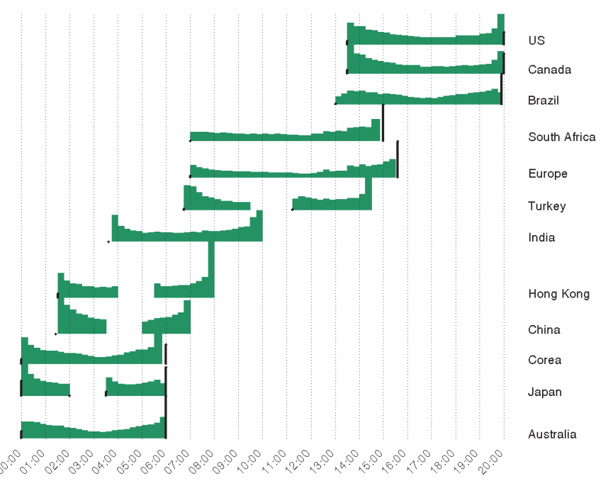
<p>The U and J shapes seen in  figure 2 should be analyzed with different causes in context:</p>
<ul>
  <li>Opening of a linked market.</li>
  <li>Release of news at a predetermined time of day on a regular basis.</li>
  <li>Computation of reference prices and if fixing phase is used for this purpose.
    <ul>
      <li>For many European funds the reference price is the closing price. India does not have a closing price and instead uses VWAP over the last half-hour of trading. 
<!---Images--></li>
    </ul>
  </li>
</ul>
<figure style="display: flex; flex-direction: column; align-items: center;">
  <img src="/assets/ch2_mm/intra_vol.png" alt="curve" width="400" />
  <figcaption>Figure 2.  Intraday volume patterns across the globe </figcaption>
</figure>

<p>Hong Kong’s volume pattern is shown to be highly dependent with the way reference price is computed.</p>

<p>Brazil’s opening hours are slow until US markets open 30 minutes later. At this time the Brazilian markets will have real price formation; Brazil’s markets are heavily dependent on the US’, instilling winter and summer hours to be more closely matched with US hours. This same market dependency can be said about South African markets and European markets.</p>

<p><strong>Effects of Volume Patterns</strong><br />
Opening of the US Markets:</p>
<ul>
  <li><em>NY shift</em>: Computed volume pattern using days where there is only a 5-hour difference between French time and US time.
    <ul>
      <li>Increase in  volume occurs when the US markets are open one hour earlier.</li>
      <li>Spikes on the third Friday of March and select months are due to expiry dates.</li>
    </ul>
  </li>
  <li><em>NY Closed</em>: Volume pattern on the days where the US market is closed but the French market is open. Activity volume is much lower.</li>
</ul>

<p>US macroeconomic news:</p>
<ul>
  <li>Immediate release of economic activity reports on volume depend on how surprising it is for the market.</li>
</ul>

<p>Equity derivatives expires:</p>
<ul>
  <li>Witching days and expiry days make investors who do not want to roll over positions unwind cash positions and generate huge volumes during certain time stamps.</li>
  <li>The exchange date settlement price (EDSP) for single stock futures and options is the closing call auction price. This is why closing fixings have large volume as well.</li>
</ul>

<p><strong>Fragmentation and Evolution of Intraday Volume Patterns</strong><br />
Market share is more important at the beginning vs end of the day. This is because beginning PFP is taking place on the primary market from unmatched opening fixing orders. As well, mature players will time SORs to not route orders to MTFs at time if not needed.</p>

<p>Chi-X’s Jan-Feb 2012 dip (below the 50% threshold) can be explained by the influx of liquidity providers who need to increase activity at the end of the day.</p>

<p>Participants unwinding their cash hedging positions at a price close to EDSP will want to trade on markets where the price will be observed to target reference prices and directly participate in its fixing with their own execution prices.</p>

<h2 id="four-main-liquidity-variables">Four Main Liquidity Variables</h2>
<p>The four main liquidity variables are:</p>
<ul>
  <li>Traded Volume</li>
  <li>Bid-Ask Spread</li>
  <li>Volatility</li>
  <li>Quoted Quantities</li>
</ul>

<p>Given the state of microstructure and associated trading offers, liquidity providers and consumers explicitly or implicitly accept to trade. The amount traded reflects fragmentation.</p>

<p><em>Offered liquidity</em></p>
<ul>
  <li>Offered liquidity serves as the counter part for traded volume as a variable for liquidity. It can be approximated as the first limit of the books.</li>
</ul>

<p><em>Book size, liquidity in the book</em>:</p>
<ul>
  <li>The book size is the average between the quantity at the best bid and at the best ask. (for smaller tick sizes several limits will need to be summed compared to larger ticks).</li>
  <li>Book size is significant for maximum tradable quantity and serves as a lower bound for traded volume. This concepts is more complex given orderbooks replenish.</li>
</ul>

<p>All in all book size is an indication of interest of liquidity providers who are ready to trade at the current prices (around mid-price).</p>

<p>The bid-ask spread is the best lowest ask and the highest buy. An instrument is less liquid if the spread is tighter and vice versa.</p>

<p>Comparing bid-ask spread  $\psi_1$ vs $\psi_2$ you will find that</p>

\[\begin{align}
\psi_i = a + b \cdot \frac{1}{\sqrt{N_i}} \cdot \sigma_i
\end{align}\]

<p>$N_i$ is the average number of traders per day. $a, b$ are constants that seem to be shared by all instruments given an asset class.</p>

<p>Using $\eta$ we can compute the bid-ask bounce to be,</p>

<!---Theorem box-->
<div style="border: 2px solid #ccc; border-radius: 8px; padding: 16px; margin: 20px 0; background-color: #f9f9f9;">
  <strong>Bid Ask Bounce</strong>
  <p>
    $$\begin{align}
    \psi_i = a + \frac{1}{\sqrt{N_i}}(b_1 \cdot \sigma_i + b_2 \cdot \eta \cdot \text{ tick})
    \end{align}$$
  </p>
</div>

<p>$\eta$ is estimated using traded price and</p>
<ul>
  <li>$N^a$ of alternations of price over the day</li>
  <li>$N^c$ of continuations of price over the day</li>
</ul>

<p>Then,</p>

\[\begin{align}
\eta = \frac{N^c}{2N^a}
\end{align}\]

<p>$\eta$ is influenced by the bid-ask bounces. The more bounces the more alternations and the smaller the parameter. If prices move randomly then $\eta$ is balanced. This parameter can be used to predict the effect of a tick change.</p>

<p><strong>Intraday Seasonalities</strong> <br />
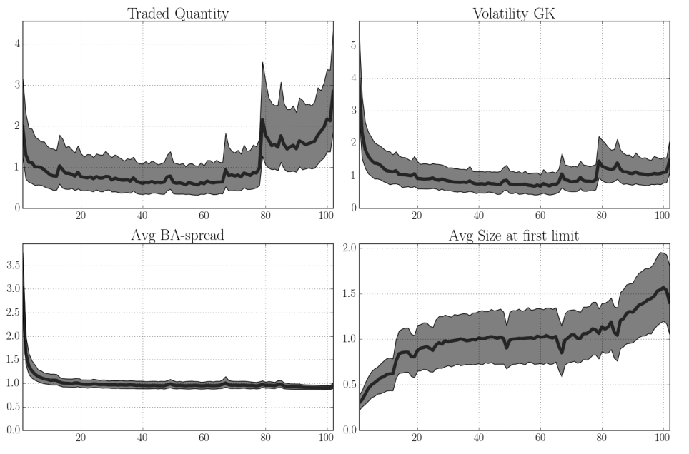
Traded volumes, bid-ask spreads, quantities at first limits, and volatility exhibit intraday patterns. They correspond to more uncertainty on the price after the opening, less activity during mid-day, and a run to end trading before the close. Scheduled events like news influence these patterns.</p>

<!---Images-->
<figure style="display: flex; flex-direction: column; align-items: center;">
  <img src="/assets/ch2_mm/intraday_vol.png" alt="cave" width="450" />
  <figcaption>Figure 3. Renormalized intraday seasonalities on Royal Dutch Shell (UK listed stock)</figcaption>
</figure>

<p>Volatility is estimated by different models such as Brownian models. Implied volatility can be used as a proxy for volatility but this measure looks at uncertainty of future prices. In the context of microstructure we need to understand the frictions of past trading activity.</p>

<p>The naive estimator of volatility is not a good estimator because of pollution of bid-ask bounce.</p>

<p>In figure 3 we see that the four curves exhibit intraday seasonality. Traded volume, bid-ask spread, and volatility are high at the start of the day. By mid day the price formation process readjusts prices and movement has calmed. By the end of the day volume increases given participants trying to close positions.</p>

<p>When bid-ask spread is large the volume on the book is rather small and vice versa. At the end of the day the spread is at its minimum and <em>when it is at its minimum the book size increases</em> to compensate.  Liquidity providers who can’t step into the spread (given its size is the tick size) will have to increase sizes at best bid and ask to provide liquidity, hence increasing the book size.</p>

<p>When the spread is stuck to one tick an increase in the book size plays a role similar to a spread decrease.</p>

<h2 id="does-more-liquidity-guarantee-a-better-market-share">Does More Liquidity Guarantee a Better Market Share?</h2>
<p>Before MiFID, transactions took place on single national exchanges where liquidity providers and investors were mandated to interact in the same place. Now, with the introduction of competition, exchanges have to attract and keep market-makers, transforming investors into connected members.</p>

<p>Market-makers are attracted through maker/taker fees. Members are attracted through connections costs.</p>

<p>The number of connected member and the satisfaction of market makers is conditional on the liquidity of the exchange</p>

<p><em>Liquid stock</em>: High volume combined with low volatility and bid ask spread.</p>

<p>Creating and maintaining a trading venue requires:</p>
<ul>
  <li>Liquidity providers</li>
  <li>Competitive bid-ask spreads</li>
  <li>Connected members</li>
</ul>

<p><strong>Bid-Ask Spread’s Influence on Liquidity</strong> <br /></p>
<ul>
  <li>The higher the volume on a trading venue the more its market share.</li>
  <li>Volatility cannot be considered as an element of market design choices for an exchange.</li>
</ul>

<p>The bid-ask spread represents the reward given to the market maker for the risk of providing liquidity.</p>

<p>The bid-ask spread is a way for exchanges to grab market share by increasing the chances the venue hosts a transaction. This is different in the US where mandates for best executions are implemented by consolidated tape.</p>

<p><strong>The Bid-Ask Spread and Volatility Move Accordingly</strong> <br /></p>

<p><em>The daily bid-ask spread increases with daily volatility.</em></p>

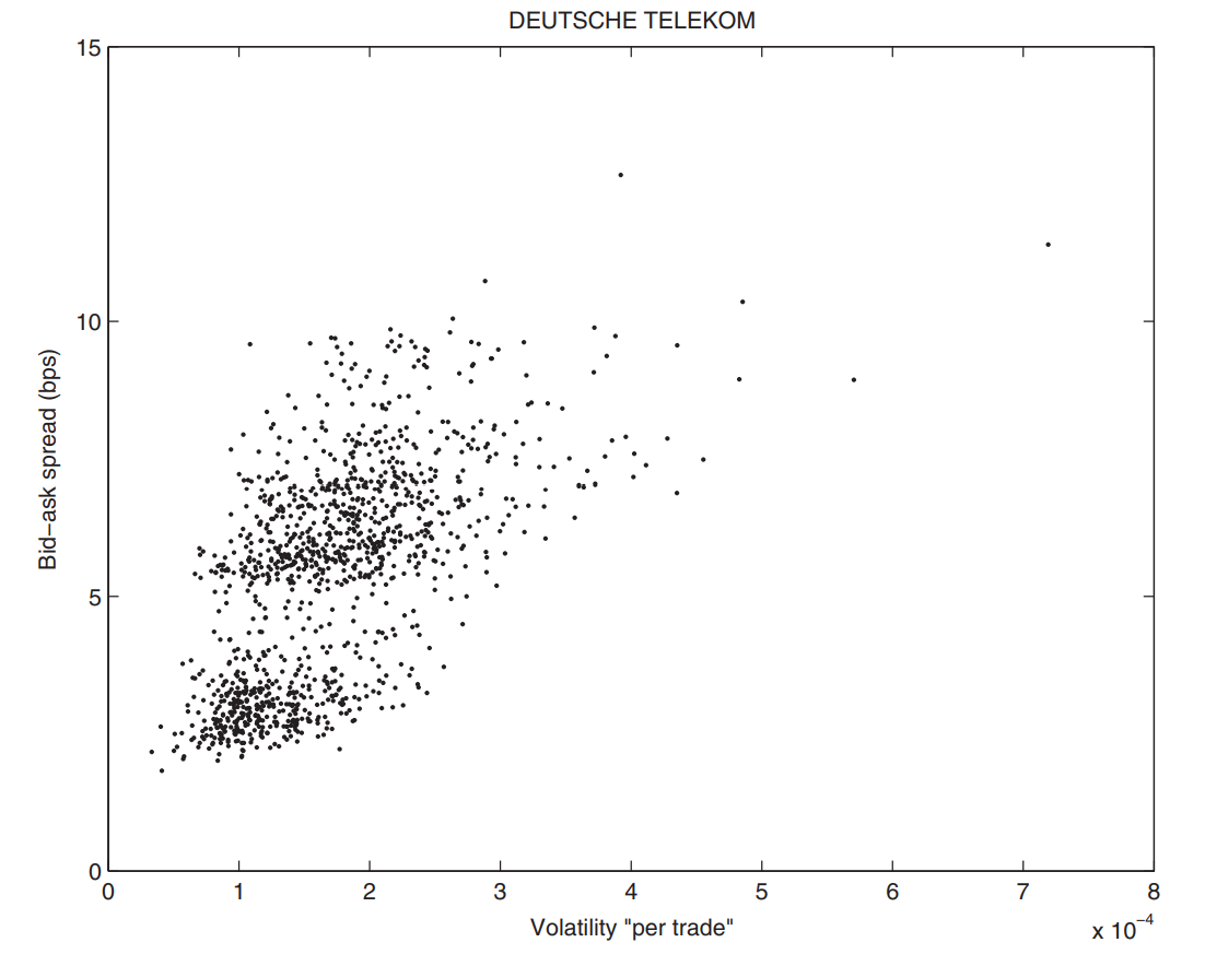
<p>The higher the volatility the higher market makers ask to compensate for their possible loses. This can be modeled with a simple linear regression where volatility can be adjusted per trade (seen in figure 4).</p>

<!---Images-->
<figure style="display: flex; flex-direction: column; align-items: center;">
  <img src="/assets/ch2_mm/vol_bid.png" alt="vol_bid" width="400" />
  <figcaption>Figure 4. Bid–ask spread and volatility per trade on Deutsche Telekom</figcaption>
</figure>

<p>For contributions of microstructure, short term intervals need to be taken into account. After the opening of the market, the market suffers through lots of noise; hence the bid-ask spread and volatility are high. Movement dies down in the middle of the day but picks up by closing because of HFTs needs to flatten residual inventory, making them accept tighter bid-ask spreads regardless of risk.</p>

<p><strong>Bid-Ask Spread and Market Share are Deeply LInked</strong> <br />
Market maker activity is more risky on less traded stocks - hence their reward is higher. The market share of a venue moves according to the quality of its bid-ask spread in relative terms.</p>

<p>Tight relative bid-ask spreads imply an increasing market share because SORs are mandated to generate transactions on the venue providing the best price.</p>

<p><strong>Exchanges Need to Show Volatility Resistance</strong> <br /> 
The dependence of the bid-ask spread on volatility is taken into account because it has impact on market makers. Because market makers have the duty to provide liquidity to other participants, they will choose markets that are resilient to relatively high levels of volatility.</p>

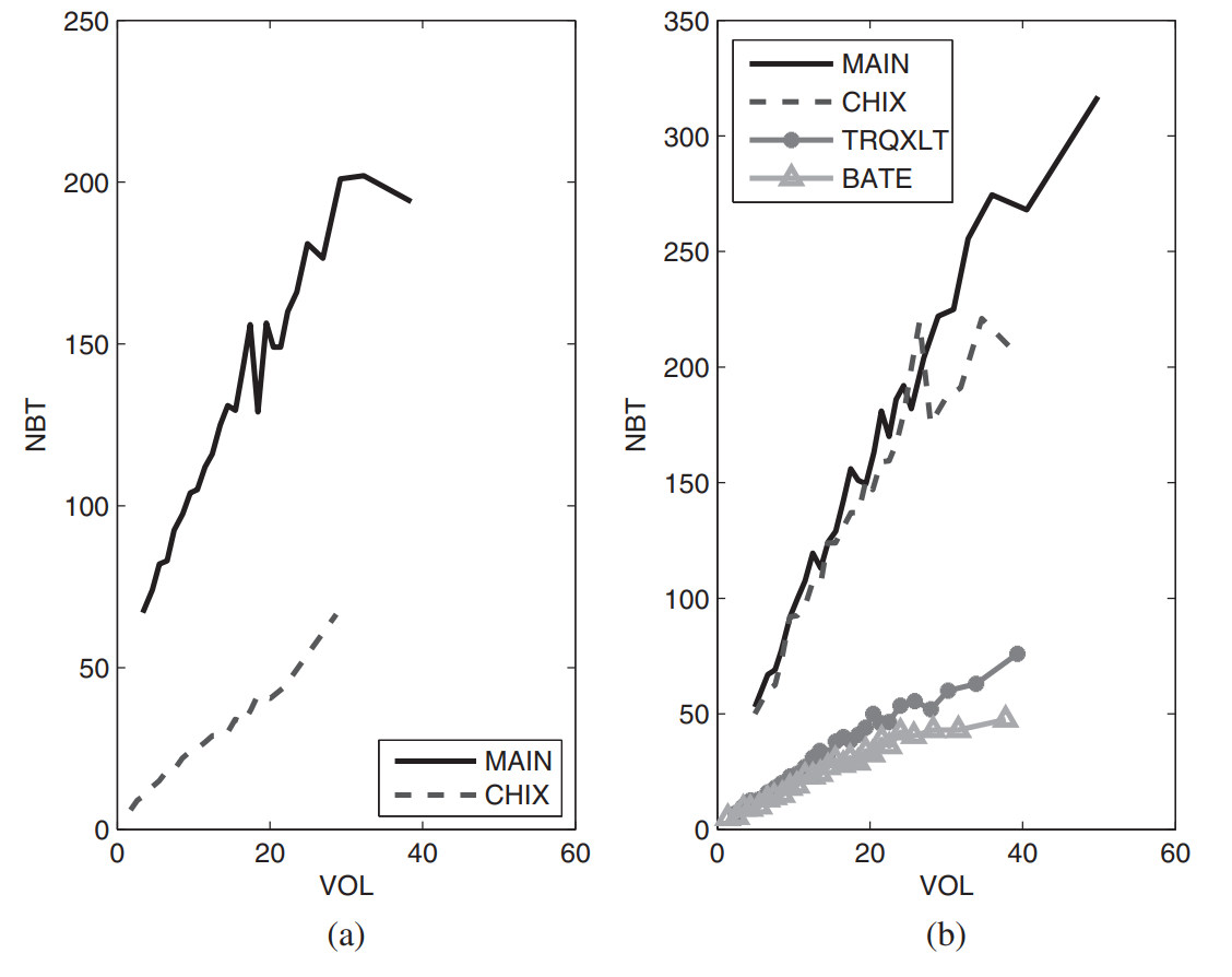
<p>Resilience can be measure with the relationship between the number of trades on a trading venue and its price volatility.</p>

<!---Images-->
<figure style="display: flex; flex-direction: column; align-items: center;">
  <img src="/assets/ch2_mm/med_linked.png" alt="med_linked" width="400" />
  <figcaption>Figure 5.  Median number of trades over quantiles of high frequency volatility for Total SA in 2008 (a) and 2012 (b)</figcaption>
</figure>

<p>In figure 5(a) the primary market has the highest slope, meaning that it offers a far higher relative number of trades during the volatile periods than other markets. The PFP tends to occur where transactions have the most resilience to volatility, hence Chi-X takes a greater part in the PFP vs. BATS and Turquoise.</p>

<p>But this behavior differs from liquid to illiquid stocks.</p>

<p>Indexes and venues can be compared using the correlation between the number of trades and high frequency volatility. This is called <em>flow reactivity</em> which dictates the hierarchy of destinations. When a venue has low flow reactivity, high frequency market makers stop offering as much liquidity as they do during calmer periods.</p>

<p>There is a strong relationship between quality of trading venue, success, and market makers that operate it. Venues have the <em>obligation to keep market makers active in order to improve market share through competitive spreads and resilience to volatility (better liquidity)</em>.</p>

<h2 id="the-agenda-of-hfts">The Agenda of HFTs</h2>

<p>The main question concerning HFTs is: Does this market design enable competition between several markets have negative externalities?</p>

<p>Fragmentation was in response to financial market monopolies  to decrease prices and  increase trading quality.</p>

<p><strong>Metric for the Balance in liquidity Among Indexes</strong> 
Turnover is chosen as a measure of heterogeneity of liquidity among stocks.</p>

<p>We can then ask the question: How well is turnover dispatched between components of indexes? Are only a few stocks responsible for activity on one index or do all components contribute to it equally?</p>

<p>The coverage metric and Gini coefficient evaluate this level of inequity.</p>

<p><em>Coverage metric</em>:</p>
<ul>
  <li>This indicates which percentage of the number of stocks is needed to realize 80% of the total turnover.</li>
  <li>This is a static viewpoint that does not take into account the shape of repartition of turnover across stocks. Repartition meaning if the 20% is concentrated over medium traded stocks or spread thinly over low activity ones.</li>
</ul>

<p><em>Gini coefficient</em>:</p>
<ul>
  <li>The Gini coefficient uses the whole repartition curve to estimate the degree of inequality among stocks.</li>
  <li>The repartition curve is found by summing all intraday turnover on each component after the components have been sorted in decreasing order and diving by sum (to normalize).</li>
</ul>

<p>The Gini index and Kolmogorov–Smirnov test is covered in chapter 1 notes. It can also be reviewed in A.9.</p>

<p>The higher the coverage or the lower the coefficient the more the investor can <em>find an equivalent quantity of liquidity on every stock of the index for a specific exchange</em>.</p>

<!---Images-->
<figure style="display: flex; flex-direction: column; align-items: center;">
  <img src="/assets/ch2_mm/repart.png" alt="repart" width="400" />
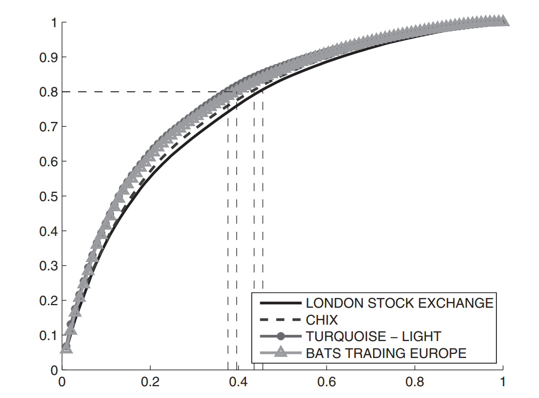
  <figcaption>Figure 6.  Repartition of turnover among FTSE 100 stocks on the four main trading venues</figcaption>
</figure>

<p>In figure 6 the turnover for 45 FTSE 100 stocks equates to 80% of the total turnover of the entire index on the LSE. By tracing a horizontal line from the y axis where it reads 80% we can find the corresponding x axis value that intersects with the repartition curve. The area under the curve multiplied by two represents the Gini index.</p>

<p>LSE’s coverage liquidity metric is around 45%. The Gini index, which indicates how far the repartition of turnover is from a uniform repartition, is equal to 0.99.</p>

<p><strong>The History of Coverage</strong> <br />
Between 2009 - 2012 coverage values increased, decreasing the discrepancies between venues. This created positive homogeneity but did not impact illiquid stocks given HFTs could not increase their activity on them given hedging and short selling is incredibly expensive with large risk.</p>

<p>With the evolution of Multilateral Trading facilities (MTFs), market share became dependent on stock liquidity. Because HFTs have higher risk when extending their activity to less liquid stocks, MTFs increase coverage for wide indexes. Therefore, HFTs extend their perimeter of action for a symbiotic relationship.</p>

<p>High frequency market makers increase uniformity among indexes coverage by spreading volume and ensure the contribution of MTFs to the price formation process by arbitrage.</p>

<p><strong>HFTs Do Not Impact All Investors Equally</strong> <br /> 
Platforms reward trading strategies that make use of the maker/taker schedule. Arbitrageurs use technology to lower inventory risk by trading very small orders very frequently.</p>

<p>The SEC definition for HFTs is as follows:</p>
<ol>
  <li>Very high speed and sophisticated computer programs for generating, routing, and executing orders.</li>
  <li>Use of co-location services and individual data feeds offered by exchanges and MTFs to minimize network and other types of latencies.</li>
  <li>Very short timeframes for establishing and liquidating positions.</li>
  <li>Submission of numerous orders that are cancelled after submission.</li>
  <li>Ending the trading day in as close to flat position as possible.</li>
</ol>

<p><strong>How HFTs Lower Spread Without Changing Execution Costs</strong> <br /></p>

<p>The effective spread is reduced on an overall basis, but the costs for other participants remain unchanged or slightly increased.</p>

<!---Images-->
<figure style="display: flex; flex-direction: column; align-items: center;">
  <img src="/assets/ch2_mm/three_cases.png" alt="repart" width="500" />
  <figcaption>Figure 7.  Three cases of the orderbook</figcaption>
</figure>

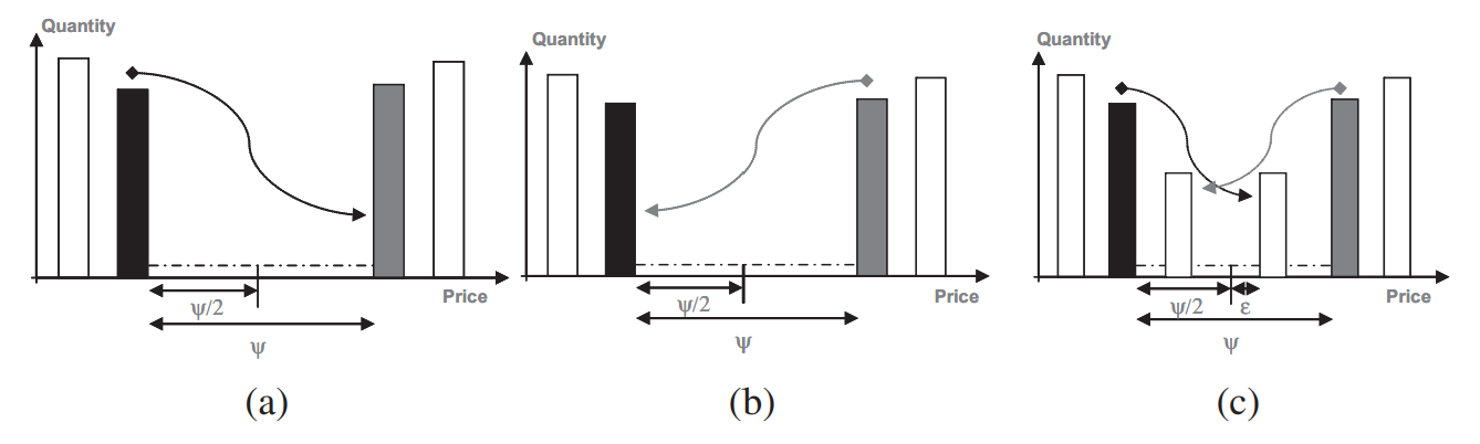
<p>If we consider a market with player A and B, seen in figure 7(a), A becomes impatient and hits player B’s price in order to trade. His cost is the bid-ask spread $\psi$.</p>

<p>In 7(b) player B becomes impatient and hits player A’s price in order to trade. His cost is the bid-ask spread $\psi$. Hence A and B will bear the cost of $\psi / 2$.</p>

<p>In 7(c) a HFT intervenes on the market and takes a position on the outside of B and the first limit against A. A hits the HFT price and his cost is slightly more: $\psi / 2 + \epsilon$. The HFT takes a new position rapidly in front of B, and since B’s order is not matched, B needs to hit the HFTs price. His cost then becomes $\psi / 2 + \epsilon$.</p>

<p>The final effective bid-ask spread is reduced since it represents slightly more than half the formal bid-ask spread. The HFT forces player A and B to become more aggressive, but given trade sizes are small, prompts other participants to fraction their orders, incurring cost. These fixed costs are unevenly distributed and lead to a deterioration in trading conditions for final investors.</p>

<p><strong>Bid-Ask Spread: Cost and Uncertainty for Investors</strong> <br />
We now consider if bid-ask spreads would have been unchanged if HFTs had not appeared. If we consider HFTs involved in $q$% of trades, the new bid-ask spread is</p>

\[\begin{align}
\psi_N = q\psi_{HFT} + (1-q)\psi_B.
\end{align}\]

<p>The proportion of HFTs among trades is assumed to be 40% and  the spreads take the values,</p>

\[\begin{align}
\psi_B = 5.41bp\\
\psi_N = 4.73bp
\end{align}\]

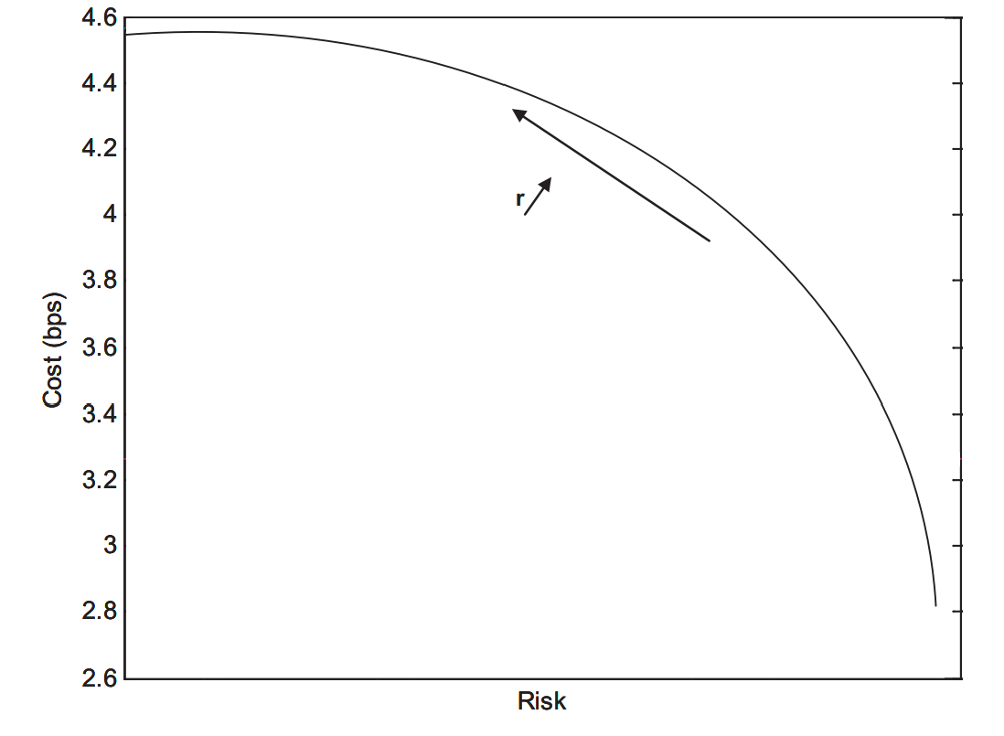
<p>For the cost $C$ the investor has to look at the probability $r$ of meeting a HFT. Three scenarios are outlined:</p>
<ul>
  <li>If the investor encounters a HFT and is willing to be aggressive the his cost is $C = \psi_{HFT} / 2 + \psi_{B} / 2$.</li>
  <li>If the investor does not encounter a HFT then his cost is $C = \psi_B$.</li>
  <li>If he does not encounter a HFT and is passive he pays $C = 0$.</li>
</ul>

<!---Images-->
<figure style="display: flex; flex-direction: column; align-items: center;">
  <img src="/assets/ch2_mm/execution.png" alt="execution" width="400" />
  <figcaption>Figure 8.  Execution cost and its uncertainty</figcaption>
</figure>

<p>In figure 8 the curve represents $C$ and the uncertainty that relates to $C$. The smaller the cost the higher the uncertainty about it (like the efficient fronter portfolio). Points on the line vary depending on the probability $r$ of meeting an HFT. Increasing this probability increases cost by reduces uncertainty.</p>

<p>For large numbers of trades the Central Limit Theorem (CLT) is used such that,</p>

\[\begin{align}
\mathbb{E}[\frac{1}{N}\sum^N_{i=1}C_i] = \mathbb{E}[C] \\
Var(\frac{1}{N}\sum^N_{i=1}C_i) = \frac{Var(C)}{N}. 
\end{align}\]

<p>The uncertainty is lower with the increase of trades.</p>

<p>The bid-ask spread is a source of cost for investors in the market. Both the expected value of this cost and the uncertainty are key figures. Depending on the number of trades and the probability of meeting an HFT actor expectation will not vary but uncertainty will significantly.</p>

<h2 id="the-link-between-fragmentation-and-systemic-risk">The Link Between Fragmentation and Systemic Risk</h2>
<p><em>Systematic risk</em> can be seen as the residual risk that is left in a portfolio when all the other risks have been hedged through all possible financial instruments.</p>

<p>Investors ask if systematic risk has increased with the rise fo HFTs. This gives way to the relationship between extra and intraday volatility. At what extent does extraday volatility effect intraday volatility?</p>

<p><strong>Overnight vs Intraday Correlation</strong> <br /> 
We examine the trends of the average intraday and overnight correlations among the components of an index.</p>

<p>Correlation spikes are often well explained by overnight ones.</p>

<p>Intraday correlation reflects to some extent the amount of co-movement between securities at intraday scale. This is an intermediary marker in the contagion process which leads microscopic causes for macroscopic effects.</p>

<p>To calculate intraday correlation:</p>

\[\begin{align}
\text{Intraday Correlation} =
\text{Corr(intraday return A, intraday return B), overnight correlation} \\
= \text{Corr(overnight return A, overnight return B)}
\end{align}\]

<p>where</p>

\[\begin{align}
\text{Intraday return} = \log(\text{close}_t)- \log (\text{open}_t) \\
\text{Overnight return} = \log(\text{open}_t)- \log (\text{close}_{t-1}) 
\end{align}\]

<p>During the night the market is organized as an auction fixing and during the day as continuos trading. Hence opening fixing is less liable to be contaminated by loud microstructure noise and tends to reflect consensus of price vs closing fixing. The overnight corrections are closer to extraday correlation.</p>

<p><strong>Flash Crash Analysis</strong> <br />
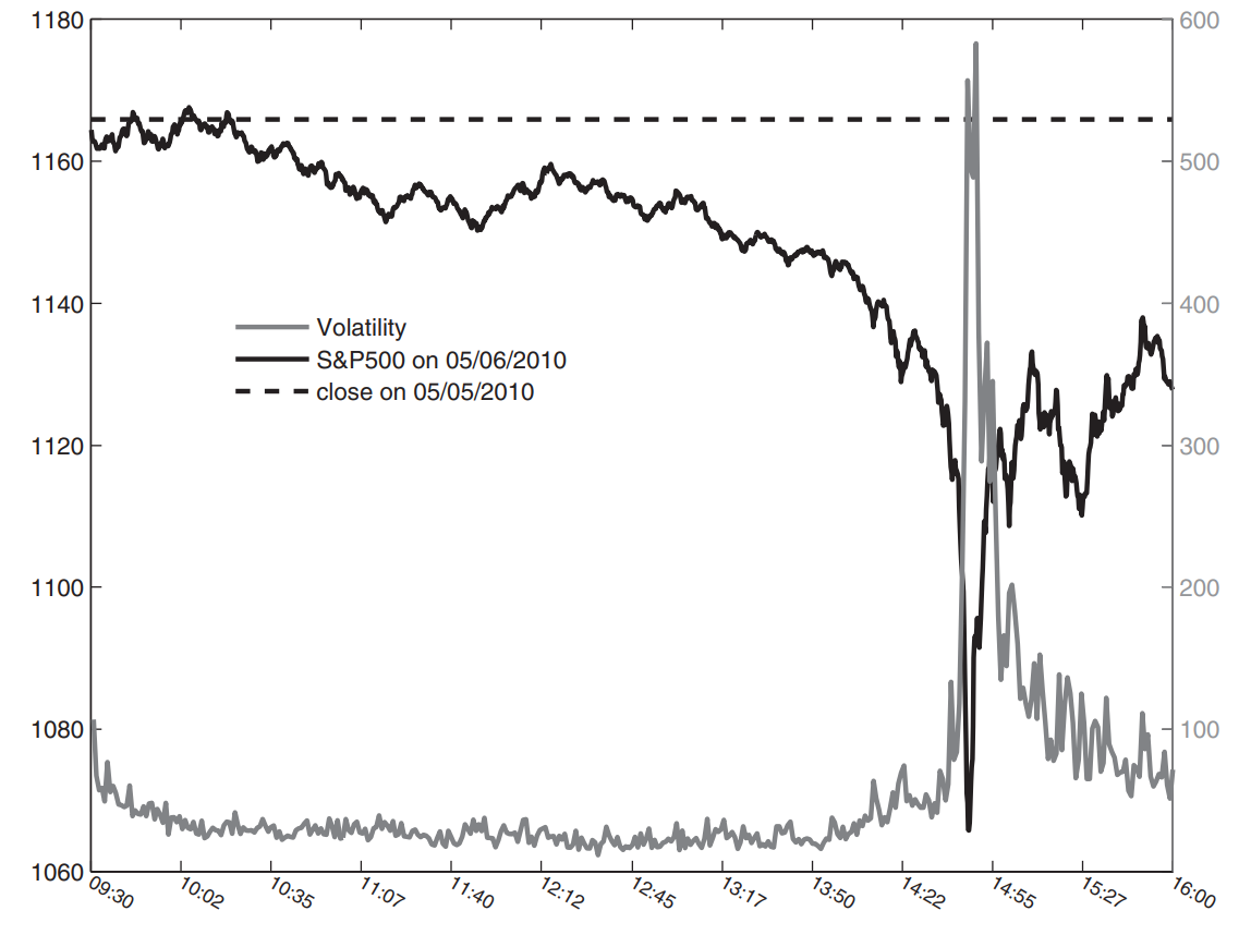
On May 6, 2012 the US stock market suffered a sudden and rapid drop following a rapid recovery.</p>

<!---Images-->
<figure style="display: flex; flex-direction: column; align-items: center;">
  <img src="/assets/ch2_mm/flash_crash.png" alt="flash_crash" width="400" />
  <figcaption>Figure 9. S&amp;P 500 and volatility among S&amp;P 500 components on May 6, 2010</figcaption>
</figure>

<p>The SEC and CFTC suggested several reasons. The large sale of US indexes on May 6th initiated by a trader who did not put a limit price on the algorithmic order caused an excess of volume that brought HFTs to hedge themselves in light of high risk that day. The snowball effect of hedging eventually returned to its starting point and caused escalations of volume while liquidity offered remained unchanged. The artificially increased volume caused traders to increase flow sent to the market and fed the vicious cycle.</p>

<p>The jump in volume in the market was followed by a large number of HFT players liquidating their positions, increasing imbalance between the demand and supply of liquidly.</p>

<p>The E-mini and SPY showed desynchronization. With the nigh volatility b=on both derivatives, this caused an interruption in the number of orders which transmitted a shock to the stock market. With a pause on orders and the re-routing of OTC orders to primary markets, the pressure on the aggressive side of the orderbook was rising.</p>

<p>As well the Liquidity Replenishment POint (LRP) that slackens the market for a period of time for liquidity to return exacerbated the imbalance between supply and demand. When LRP is triggered all aggressive orders are rerouted to other exchanges - the immediate effect of removing passive liquidity in the NYSE but retaining aggressive liquidity is disastrous.</p>

<p><strong>Systematic Risk and Circuit Breaking</strong> <br /> 
The Flash Crash raised new concerns about the stability of markets. Automation of market making seems to allow liquidity providers to suffer from less adverse selection (because they process information faster). If adverse selection of market makers is a stabilizing force for the PFP, then it can be expected that the more aware adverse selection providers are, the less stable the markets.</p>

<p><strong>Circuit Breakers</strong> <br /> 
Circuit Breakers may be crucial protection against sudden demand of liquidity by market participants. In principle there is a need to stop the PFP in a local or global scale. For a micro scale how can we differentiae between usual liquidity imbalance vs an unusual one that halts trading? Is it even a good idea to halt trading?</p>

<p>Circuit breaks are expected:</p>
<ul>
  <li>To be activated ini case of liquidity imbalance, but all of them loo at prices. Instead looking at the conjunction of price moves ad poor liquidity can help define more adequate thresholds.</li>
  <li>To be activated in case of abnormal price swings. One should take into account two levels of volatility (daily and intraday variations) using intraday seasonalites.</li>
  <li>Instruments whose prices are indexed on halted tradable assets should be halted when trading on the latter has been halted. This ensures fair trade.</li>
  <li>Highly correlated instrument should be halted to stop propagation of trading impact.</li>
  <li>Synchronization of circuit breakers should be considered and their propagation effect.</li>
</ul>

<h2 id="beyond-equity-markets">Beyond Equity Markets</h2>
<p><strong>Trading Futures</strong> <br />
Futures are highly electronified. They have no call auction and participants have to agree on liquid hours during which they trade. Futures usually correlate to trading on equities but some studies suggest PFP on futures leads PFP on their components. 
Tick sizes of futures are usually larger and cause lots of bid-ask bounce and price reversion. Sizes of first limits of futures are therefore much larger compared to equities.</p>

<p>Future markets are almost not fragmented given post-trading processes would be more complex if fragmented.</p>

<p><strong>Trading Options</strong> <br />
The post-trading process on options is more complex than futures.  US options markets are fragmented (European ones are note). The current challenge for options markets is to attract market makers given they only post liquidity in limit orderbooks and the buyside consumes liquidity.</p>

<p><strong>Trading Fixed-Income Products</strong> <br />
Fixed income products cover a wide variety of instruments: swaps, bonds, foreign exchange credit default swaps, ect. These highly liquid products are traded on electronic platforms close to equites.</p>

<hr />
<p>Chapter 2 notes are complete!</p>

<p>The penultimate chapter of <em>Market Microstructure in Practice</em> will focus on optimal organizations for optimal trading - specifically targeting trading structure, market impact measurements, and the PFP dynamics on orderbooks.</p>]]></content><author><name>Brook Chuang</name></author><category term="Market Microstructure" /><summary type="html"><![CDATA[In Chapter 2 of Market Microstructure in Practice by Lehalle and Laruelle we explore the nuances of fragmentation by looking at volume curves, the four main variables of liquidity, market share’s effects on spread, and the agenda of HFTs.]]></summary></entry><entry><title type="html">Walton Ford’s World: Delirium of Animal and Man</title><link href="https://brookchuang1111.github.io/2025/04/20/walton-ford.html" rel="alternate" type="text/html" title="Walton Ford’s World: Delirium of Animal and Man" /><published>2025-04-20T00:00:00+00:00</published><updated>2025-04-20T00:00:00+00:00</updated><id>https://brookchuang1111.github.io/2025/04/20/walton-ford</id><content type="html" xml:base="https://brookchuang1111.github.io/2025/04/20/walton-ford.html"><![CDATA[<p>I feel the beast’s stance in my throat - I feel the tension of his hind legs in my spine.</p>

<p>Fenrir’s large black body covers the canvas while a pale limb in the corner entices the jaws of the beast to sever it completely off the limb. He is bound by a silky pink ribbon called Gleipnir, whose strength seems inconsequential next to the hulking figure of the animal.</p>

<!---Images-->
<figure style="display: flex; flex-direction: column; align-items: center; padding-top: 20px; padding-bottom: 20px;">
  <img src="/assets/walton_ford/wolf.png" alt="wolf" width="400" />
  <figcaption style="width: 400px; text-align: center;">Figure 1. Gleipnir, 2012 watercolor, gouache, ink, pencil on paper. Painting by Walton Ford courtesy of the Kasmin Gallery</figcaption>
</figure>

<p>The painting is both mythic and unsettling, blurring the line between predator and prey, reality and fable. This tension lies at the heart of Walton Ford’s piece <em>Gleipnir</em>, where the fantastical collides with naturalist narratives for a spin of the unusual.</p>

<p>For the American artist Walton Ford, this is commonplace. Ford’s art is vivid and wild, pushing the viewer to find the storyline embedded into his subjects. His landscapes seems to grapple with the confines of their canvas, exhibiting  the punishing nature of animal order and unabashed pride for the untamed.</p>

<p>Selfishly, in hopes of bringing some of his genius with me, I had went to CVS to print out a selection of his work before the start of junior year. My favorite out of the set, <em>Delirium</em> (2004), was a vertical painting of a bald eagle in flight, intended to hang in my room above my desk. When my roommates inquired about my selection of posters, I ecstatically showed them the poster of the bird.</p>

<p><em>“Oh so your room is going to be hunting themed?”</em></p>

<p>No you cretin, it is not. Safe to say they sorely misunderstood the subject, so I relocated the poster to my childhood bedroom for the pleasure of more discerning eyes.</p>

<p>But for the more perspicacious reader, it would be my honor to introduce the history, background, and interpretations of <em>Delirium</em> (2004), and why it represents such a piece of brilliance to me.</p>

<p>To start, we must turn our attention to an ornithologist by the name of John James Audubon.</p>

<h2 id="the-natural-order-of-birds-skulls-and-race">The Natural Order of Birds, Skulls, and Race</h2>
<blockquote>
  <p>“I must acknowledge that as I watched his eye, and observed his looks of proud disdain, I felt towards him not so generously as I ought to have done” - John James Audubon, 1835</p>
</blockquote>

<p>John James Audubon was a naturalist and ornithologist credited for documenting and introducing the public to the biodiversity of America. His seminal <em>The Birds of America</em> was his magnum opus and response to his life’s objective of illustrating all bird species in America.</p>

<p>Comprising 435 life-size prints, <em>The Birds of America</em> graces museums across the country, reverently coddled in air conditioned rooms and treated to the silk gloves as museum conservatives riffle through their pages. Audubon too is graced with such admiration; buildings, neighborhoods, and streets sport his name - a testament to his contributions to science and a promise to withhold his legacy.</p>

<!---Images-->
<figure style="display: flex; flex-direction: column; align-items: center; padding-top: 20px; padding-bottom: 20px;">
  <img src="/assets/walton_ford/jja.png" alt="jja" width="300" />
  <figcaption style="width: 300px; text-align: center;">Figure 2. John James Audubon. Painting by John Syme courtesy of White House Historical Association</figcaption>
</figure>

<p>But every coin has two sides. The naturalist was a staunch anti-abolitionist who embraced racial pseudoscience. Famously, Audubon collected five skulls of the unburied on a battlefield during the Texas War to be sent to Samuel Morton. Morton used these skulls to “define racial categories and hierarchies” by studying cranial differences that he thought to define human races. Unsurprisingly, Morton thought that the race with the largest brains, and consequently had the highest intelligence, belonged to Caucasians<sup id="fnref:1" role="doc-noteref"><a href="#fn:1" class="footnote" rel="footnote">1</a></sup><sup id="fnref:2" role="doc-noteref"><a href="#fn:2" class="footnote" rel="footnote">2</a></sup>.</p>

<!---Images-->
<figure style="display: flex; flex-direction: column; align-items: center; padding-top: 20px; padding-bottom: 20px;">
  <img src="/assets/walton_ford/skull.png" alt="skull" width="300" />
  <figcaption style="width: 300px; text-align: center;">Figure 3. Lithograph from Samuel George Morton, Crania Americana. F. Davis (engraver), Public domain. Courtesy of Wikimedia Commons </figcaption>
</figure>

<p>Audubon “had no stance on slavery” according to earlier biographers by…owning slaves. It is known that the Audubon household continually bought and sold slaves as financial constraints allowed.</p>

<p>Audubon never saw people of color, African Americans and the Indigenous, as equals. Even when outsourcing assistance and observations to communities who were adept with the local flora and fauna, John Audubon refused to acknowledge or credit their expertise. Instead, he coined multiple racially charged short stories depicting Black men as menacing and dangerous, hoping to captivate readers with the ‘savageness’ of the ‘other race’.</p>

<p>It is still not understood if Audubon was mixed race having self cited (and lied) about his mothers European origins<sup id="fnref:3" role="doc-noteref"><a href="#fn:3" class="footnote" rel="footnote">3</a></sup>.</p>

<h2 id="trapping-a-golden-eagle">Trapping a Golden Eagle</h2>
<p>According to the New England Journal of Aesthetic Research, “…on February 24, 1833, Ethan Allen Greenwood asked Audubon to help him identify a live eagle he purchased from a man who hunted fox with spring traps in New Hampshire’s White Mountains.”</p>

<p>Audubon recounts his experience of setting the trap and waiting for it to catch in his 1835 <em>Ornithological Biography</em>, citing by the morning the bird was caught by one of its talons, notwithstanding a struggle. Audubon convinced Greenwood to sell the 3-foot-long female golden eagle to him, hoping to capture it’s 7-foot wingspan in his <em>The Birds of America</em> etchings<sup id="fnref:4" role="doc-noteref"><a href="#fn:4" class="footnote" rel="footnote">4</a></sup>.</p>

<p>In his biography Audubon oscillated between wanting to set the bird free “might he return to his native mountains…spread out his broad wings and sail away towards the rocks of his wild haunts” or pin his wings onto a board “for the express purpose of shewing you his semblance”.</p>

<p>The more he observed the bird, the more his ambivalence grew, and in the end, Audubon’s own fever to capture the bird’s natural elegance and pride won out over “the more generous design of setting him at liberty”.</p>

<p>The next day he locked the bird in a small shed, sealing it with blankets and a pan of charcoal. He waited for the bird to inhale the fumes and suffocate, listening for the telltale sign of its body falling off its perch.</p>

<p>After hours of waiting Audubon finally checked on the bird - only to find its unflinching eyes staring back at him. This time, he intensified his efforts by adding sulfur to the shed to a point of unbearability even for himself. But alas the bird still lived, so Audubon, as a last resort, pierced the bald eagle’s heart with a pointed piece of steel. His “proud prisoner instantly fell dead, without even ruffling a feather”.</p>

<p>While working on the painting of the dead pinned golden eagle, Audubon was “suddenly seized with a spasmodic affection”. The stroke rendered much of his lip paralyzed and his hands unusable.</p>

<!---Images-->
<figure style="display: flex; flex-direction: column; align-items: center; align-items: center; padding-top: 20px; padding-bottom: 20px;">
  <img src="/assets/walton_ford/eagle.png" alt="eagle" width="300" />
  <figcaption style="width: 300px; text-align: center;">Figure 4. John James Audubon. Courtesy of the New York Historical Society</figcaption>
</figure>

<h2 id="the-descent-into-delirium">The Descent Into Delirium</h2>
<p>In <em>Delirium</em> (2004), painted by Walton Ford, we see the same bald eagle from Audubon’s illustrations. Her chest heaves from the metal spike driven into her heart and she chokes on the noxious fumes of charcoal and sulfur from the shed. Yet, even chained onto her perch, she is free from death. On the bottom left we see a rendition of Audubon lying on the snowy ground. He is dead, supposedly succumbing to the stroke that almost took his life in 1833.</p>

<!---Images-->
<figure style="display: flex; flex-direction: column; align-items: center; padding-top: 20px; padding-bottom: 20px;">
  <img src="/assets/walton_ford/walton_ford.png" alt="walton_ford" width="400" />
  <figcaption style="width: 400px; text-align: center;">Figure 5. John James Audubon. Courtesy of the New York Historical Society</figcaption>
</figure>

<h2 id="the-folly-of-animal-and-man">The Folly of Animal and Man</h2>
<p>This painting is striking to me on so many levels. The bird seems to cry out into the snowy landscape, avenging her past reality to set herself free from the chains of human brutality. She transcends her bindings as she escapes with her shackles.</p>

<p>Her life in the hands of her prisoner is nothing more than an accessory of human greed. Her captor, in hopes of capturing her animal presence for himself, intends to discard her body, letting her rot as he parades his imposed image of her. He forces a reinvention of the bird through his illustration, and to make sure his representation is superior, kills her. He trifles with the idea of mercy, but in his mind only one can exist, and with the power to terminate others, willingly does so.</p>

<p>But Walton Ford punishes Audubon for his cruel folly by reversing their subject’s interactions with death. Balancing the scales, he allows for one moment in time, for an irrational - <em>delirious</em> - instance, to let animal triumph over man. But the bird is not freed unscathed as she flees with the accessories of chains on her legs and a spike through her heart.</p>

<p>She herself is crazed from the smoke and realistically faces demise. Instead of her wings tacked to a board, her body will be pinned by the gravity of death. Her delirium is inevitable - her strength to hold out among the smoke is foolishness. Ford gives her the moment of success, but illustrates her impending doom on the horizon of her new chance of life.</p>

<p>In contrast to Ford’s <em>Delirium</em>, Audubon’s <em>Golden Eagle</em> is staid in nature. It’s a polite rendition of a majestic eagle that is barely off the ground. Ford understands these absences of - ironically - life, by foiling his painting with Audubon’s.</p>

<p>Ford’s eagle faces the other way, her wings are open, and instead of clutching sustenance in her talons, is bound by the metal of her captor. Instead of pandering to Audubon’s self eulogization of his adventurous acts - seen by his own self portrait in the landscape straddling a tree and wrangling with birds - Ford depicts Audubon inflicted by his own actions, too blind to see past his <em>delirium</em> of conquering the landscape around him to feel his heart fail.</p>

<!---Images-->
<figure style="display: flex; flex-direction: column; align-items: center; padding-top: 20px; padding-bottom: 20px;">
  <img src="/assets/walton_ford/background_jja.png" alt="background" width="300" />
  <figcaption style="width: 300px; text-align: center;">Figure 6. John James Audubon. Courtesy of the New York Historical Society</figcaption>
</figure>

<p>I like to think of Walton Ford’s revival of the <em>Golden Eagle</em> as a metaphorical unraveling of John James Audubon’s pursuit of dominance in race, achievement, and intellectualism.</p>

<p>Audubon’s foray into conquering mother nature is not unlike his campaign for racial hierarchy. By trying to tame the wilderness and natural order around him, Audubon tries to mimic the superiority he finds throughout his racial rhetoric by wrestling with his subject’s nature in hopes of molding their presence under his own.  He, the artist, wields the brush but also the sword - two instruments he uses to reroute and rewrite history.</p>

<p>In the end delirium is inflicted on both bird and human - a small reprieve of balance that Ford allots us among the scenery of human barbarity.</p>

<hr />
<div class="footnotes" role="doc-endnotes">
  <ol>
    <li id="fn:1" role="doc-endnote">
      <p><a href="https://www.science.org/content/article-scientist-built-collection-human-skulls-should-we-still-study-them">The Ghost in the Museum</a> <a href="#fnref:1" class="reversefootnote" role="doc-backlink">&#8617;</a></p>
    </li>
    <li id="fn:2" role="doc-endnote">
      <p><a href="https://commonplace.online/article/audubons-human-skulls/">Audubons Human Skulls</a> <a href="#fnref:2" class="reversefootnote" role="doc-backlink">&#8617;</a></p>
    </li>
    <li id="fn:3" role="doc-endnote">
      <p><a href="https://www.audubon.org/news/the-myth-john-james-audubon">The Myth of John James Audubon</a> <a href="#fnref:3" class="reversefootnote" role="doc-backlink">&#8617;</a></p>
    </li>
    <li id="fn:4" role="doc-endnote">
      <p><a href="http://aesthetic.gregcookland.com/2007/01/audubon-in-boston_27.html">Audubon in Boston</a> <a href="#fnref:4" class="reversefootnote" role="doc-backlink">&#8617;</a></p>
    </li>
  </ol>
</div>]]></content><author><name>Brook Chuang</name></author><category term="Art" /><summary type="html"><![CDATA[I feel the beast’s stance in my throat - I feel the tension of his hind legs in my spine.]]></summary></entry><entry><title type="html">Chapter 1: Market Microstructure in Practice</title><link href="https://brookchuang1111.github.io/2025/04/19/ch1-mm.html" rel="alternate" type="text/html" title="Chapter 1: Market Microstructure in Practice" /><published>2025-04-19T00:00:00+00:00</published><updated>2025-04-19T00:00:00+00:00</updated><id>https://brookchuang1111.github.io/2025/04/19/ch1-mm</id><content type="html" xml:base="https://brookchuang1111.github.io/2025/04/19/ch1-mm.html"><![CDATA[<p>Like a gremlin searching for gold, sometimes I scour the internet for recommended textbooks and literature on stack exchange or reddit. It gives me perverse joy to hoard these little nuggets of knowledge in a  text file on my computer, but alas, the list is too long for me in good conscious to keep stockpiling my spoils of online swashbuckling. I’ve begun the process of whittling my ‘tbr’ down with a gem called <em>Market Microstructure in Practice</em> by Lehalle and Laruelle.</p>

<p>Touted as a beginner friendly introduction to microstructure and its mechanisms, <em>Market Microstructure in Practice</em> primarily focuses on European market timelines and the evolution of Markets in Financial Instruments Directive (MiFID) regulation. Even if some microstructure design is not directly applicable to US counterparts, it’s still a very interesting read that has benefited my understanding.</p>

<p>I’ve decided to split this book into three separate posts, each dedicated to its own chapter. This series of blog posts aims to compress all my hand written notes and concepts introduced in <em>Market Microstructure in Practice</em> into an abridged notebook of sorts. I’ve outlined important concepts and some technical appendix insights that I found interesting and applicable while skipping some eulogies on the history of European markets and the birth of MiFID. Happy reading!</p>

<p>Below you can find a pdf of the textbook and my notes:</p>
<ul>
  <li><a href="/assets/market_micro/mm_textbook.pdf">Market Microstructure in Practice</a></li>
  <li><a href="/assets/market_micro/Ch_1_mm.pdf">Chapter 1 Notes</a></li>
  <li><a href="/assets/market_micro/Ch_2_mm.pdf">Chapter 2 Notes</a></li>
  <li><a href="/assets/market_micro/Ch_3_mm.pdf">Chapter 3 Notes</a></li>
</ul>

<!---Images-->
<figure style="display: flex; flex-direction: column; align-items: center;">
  <img src="/assets/market_micro/heist.png" alt="heist" width="400" />
  <figcaption>Spoils of another kind: Lost jewels of the Dresden jewelry heist</figcaption>
</figure>

<hr />

<h2 id="liquidity-in-question">Liquidity in Question</h2>
<p><em>Market Impact</em>: If information symmetry occurs between buyers and sellers, sellers offer to sell at worse prices if the buyer is not stealthy enough.</p>

<p><em>Bid-ask spread</em>: Is the distance between bid and ask price.</p>

<p><em>Slices</em>: When an investor is seeking liquidity given a large order they will have to splice such order through venues. Optimal slicing is in reference to an optimal trading theory.</p>

<p><em>Decay</em>: Decay of market impact serves to answer the question - if I consume liquidity on an asset at time $t$ how much time is needed for the price to revert?</p>

<p><em>Synchronization</em>: Large buy orders can be obscured with sell orders if there are high levels of synchronization. Hence, market impact of a large order is the average over enough market configurations.</p>

<p><em>Price Formation Process (PFP)</em>: Buying or selling pressure that is not consistent with market participant consensus will only generate a temporary impact. The opposite is true for aligning motives of participants.</p>

<p><em>Microstructure of a Market</em>: Defined as the way different traders share their responsibilities and roles.</p>

<p><strong>How the Market Consumes Liquidity</strong> <br />
Regulatory changes in 2005 have lead to new price formation processes that have shaped the market landscape. Now, HFTs act as market makers, a consequence of fragmentation within venues and products.</p>

<p>Because liquidity bridges need to be established to ensure orders are filled, arbitrageurs (HFTs) will take half the difference of the bid-ask spread and improve the level of information. Acting as information delegates, the price of HFTs adding to the fragmentation of markets is the increased flexibility of cross-trading between venues.</p>

<p><strong>The Price Formation Process</strong><br />
Driven by information, the price formation process is a paradox of its own. Sharing information is adverse for an investor, yet it is essential to use information from other participants to make informed trades.</p>

<p>In the US this conundrum has manifested into regulations across asset classes. For fixed income and equities markets, the Centralized Limit Order Book (CLOB) or Request for Quotes (RFQ) is used. The differences are aggregated below.</p>

<p>RFQs:</p>
<ul>
  <li>Bilateral</li>
  <li>Trader has fundamental information and dealer has information on flows (asymmetry of information)</li>
  <li>Trades are more exposed to <em>opportunity cost</em> while dealers are exposed to <em>adverse selection cost</em></li>
  <li>Market makers widely use conditional orders RFQs to standardize refusal to trade.</li>
  <li><em>Stalled quotes</em> are more present</li>
</ul>

<p>CLOBs:</p>
<ul>
  <li>Multilateral</li>
  <li>Participants are exposed to both <em>opportunity cost</em> and <em>adverse selection cost</em> depending on limit or market order</li>
  <li><em>Vanishing liquidity</em> is more present</li>
</ul>

<p><strong>European Market Fragmentation</strong><br />
In the US,  options are traded electronically or by using limit and market orders. This multilateral approach differs from European regulation which instead hinges on fragmentation of Central Counter Parties (CCPs) that make it virtually impossible to net-zero buy and sell the same option on different venues. Without normalization of CCPs, competition on the derivatives market is impossible.</p>

<p>When the Markets in Financial Instruments Directive (MiFID) was created in 2007, the European Union sought to change equities markets by liberalizing trading venues and creating a ‘best execution policy’. However, the application of the directive was surprising - liberalization created only a small number of alternative trading venues (Chi-X, Turquoise, BATS Europe, NASDAQ-OMX) which created high levels of competition - splitting markets into niches.</p>

<p>The ‘best execution policy’ was a matter of offering consolidated access to liquidity by both passive and aggressive orders through Broker Crossing Networks (BCNs), Smart Order Routers (SORs), and others.</p>

<p><strong>The Importance of Market Microstructure</strong><br />
At its core, market microstructure generates the price formation process. This process is the “heart of capitalism” that balances supply and demand through the context of information. The more information available to trades, the better the PFP becomes. Conversely, information leakage and front running can create negative price impacts.</p>

<p>The general consensus of the PFP is that it encompasses each trade occurring in the market combined with “fair price” of the listed asset. This can be split into two phases,</p>
<ul>
  <li>Phase 1 deals with the impact of price given movement with buys and sellers, liquidity consumers and takers. This is coined the <em>immediate price impact</em>.</li>
  <li>Phase 2 consists of liquidity returns in concordance with spread and fair price. The decay of impact from these liquidity behaviors is also known as the <em>resilience</em> of the limit orderbook.</li>
</ul>

<h3 id="fluctuations-of-market-shares-a-first-look-at-liquidity">Fluctuations of Market Shares: A First Look at Liquidity</h3>
<p><strong>Levels of Market Fragmentation</strong> <br /></p>
<ul>
  <li>Market operators</li>
  <li>Trading Venues</li>
  <li>Orderbooks</li>
  <li>Orders themselves</li>
  <li>Technology 
<!---$\mathcal{M}^k(n) = \frac{\sum_{t_1 \leq \tau^k_l \leq t_2}P^k_lV^k_l \times \mathbb{1}_n(\delta^k_l)}{\sum_{t_1 \leq \tau^k_l \leq t_2}P^k_lV^k_l}$--></li>
</ul>

<!---Theorem box-->
<div style="border: 2px solid #ccc; border-radius: 8px; padding: 16px; margin: 20px 0; background-color: #f9f9f9;">
  <strong>Market Share</strong>
  <p>
    Let $M$ be the number of transactions that took place from $t_1$ to $t_2$ over $N$ venues. If $l$ is each individual trade then the price for each trade is $P_l$ for volume $V_l$ at time $\tau_l$. 

    $\delta_1=n$ is the number of trades occurring on individual venue $n$ (where this value is 1 in the indicator function). 

    The market share of venue $n$ on stock $k$ is given as 

    $$\begin{align}
    \mathcal{M}^k(n) = \frac{\sum_{t_1 \leq \tau^k_l \leq t_2}P^k_lV^k_l \times \mathbb{1}_n(\delta^k_l)}{\sum_{t_1 \leq \tau^k_l \leq t_2}P^k_lV^k_l}
    \end{align}$$
  </p>
</div>

<p>When price of stock $k$ is relatively constant such that $\forall l: P^k_l \approx P$, we can reformulate market share as</p>

\[\begin{align}
\mathcal{M}^k(n) \approx \frac{\sum_{t_1 \leq \tau^k_l \leq t_2}V^k_l \times \mathbb{1}_n(\delta^k_l)}{\sum_{t_1 \leq \tau^k_l \leq t_2}V^k_l}
\end{align}\]

<div style="border: 2px solid #ccc; border-radius: 8px; padding: 16px; margin: 20px 0; background-color: #f9f9f9;">
  <strong>Market Share per Trade</strong>
  <p>
    To compute the market share per trade we can divide over total trades $T$, 
    $$\begin{align}
      \mathcal{M}^k_T(n) \approx \frac{\sum_{1 \leq l \leq T} \mathbb{1}_n(\delta^k_l)}{T}
    \end{align}$$
  </p>
</div>

<p>If we understand that fixing auctions change market share (more on this later), we take into account the monopoly the venue has over said auction. If venue $\mathcal{T_n}$ has an average market share of $m(n)$ during a fixing auction with weight $p$ of overall venue activity and average daily turnover $\mathbb{T} = \sum_{1 \leq l \leq T}P^k_lV^k_l$, then the average market share of a fixing auction is</p>

\[\begin{align} 
    \mathcal{M}(n \text{; ex-fixing}) \approx \frac{(1-m(n))p \times \mathcal{M}(n)\mathbb{T}}{(1-p)\mathbb{T}} \\ 
    \approx \frac{1-m(n)p}{1-p} \times \mathcal{M}(n \text{; all included}) 
\end{align}\]

<p><strong>Market Weights</strong><br />
When computing the market share of multiple stocks we look at weighting each stock by daily turnover. We can represent our market share equation as,</p>

\[\begin{align}
    \mathcal{M}^{1, \dots, K}(n) = \frac{\sum_{1 \leq k \leq K}\mathbb{T}^k\mathcal{M}^k(n)}{\sum_{1 \leq k \leq K}\mathbb{T}^k}
\end{align}\]

<p>Weighting by market share of of stock $k$ according to weight $w_k$ in a given index $J$ is given by</p>

\[\begin{align}
    \mathcal{M}^{J}(n) = \sum_{k \in J}w_k \times \mathcal{M}^k(n)
\end{align}\]

<p>The index is often proportional to the market capitalization of the stock and is not usually interpreted with daily turnover.</p>

<p><strong>Measuring Metric Adequacy</strong><br /> 
<em>Analyze the positioning and revenue of each trading venue.</em></p>
<ul>
  <li>The market share (all included) can be important even in terms of venue.</li>
</ul>

<p>*Measuring the probability when a trade occurs for security $k$ is on venue *$\mathcal{T}(n)$.</p>
<ul>
  <li>Instead of summing fixing auctions with the continuous ones, use market share during the fixing auctions and ex-fixing as separate indicators.</li>
</ul>

<p><em>Measuring the probability that, when a unit of currency (euro, dollar) is traded on security k, it is on trading venue</em> $\mathcal{T}(n)$.</p>
<ul>
  <li>The classical market share value $\mathcal{M}^{k}(n)$ is the best given we want to make one measurement during the fixing auction and another for intraday.</li>
</ul>

<p><strong>Appendix A.8. Estimation of Proportion and its Confidence Intervals</strong><br />
In microstructure we have to estimate proportions and probabilities using a binomial distribution (collection of bernoulli trials). To estimate the success the probability of success we use the empirical mean of the trials where $\hat{p} = \frac{1}{n}\sum^n_{k=1}X_k$. This unbiased estimator ($\mathbb{E}[\hat{p}]=p$) and variance $Var(\hat{p}) = \frac{p(1-p)}{n}$.</p>

<p>Given SLLN (Strong Law of Large Numbers) the estimation converges to $p$ as $n \to \infty$. By the central limit theorem (CLT), the empirical mean converges to a normal distribution. With a level of $1-\alpha$ we can approximate a confidence interval of $p$ such that,</p>

\[\begin{align}
  \hat{p} \pm z_{1-\alpha/2}\sqrt{\frac{\hat{p}(1-\hat{p})}{n}}
\end{align}\]

<p>where $z_{1-\alpha / 2}$ is the $1-\alpha / 2$ percentile of a standard normal distribution.</p>

<h3 id="first-attempts-of-fragmentation">First Attempts of Fragmentation</h3>
<p>A simple statistic to follow the fragmentation of European markets is the market share of the historical markets on each main index of each country. Given the increased competition and decreased market share, MiFID’s foray into fragmentation:</p>
<ul>
  <li>Halted the monopolistic position of historical exchanges</li>
  <li>Promoted pan-European microstructure</li>
  <li>Created LSE Group</li>
  <li>Merged Chi-X and BATS</li>
</ul>

<p>These niche markets offer two specific mixes of liquidity:</p>
<ul>
  <li><em>Natural liquidity</em>: comes directly from investors buying and selling for medium to long-term held positions.</li>
  <li><em>Opportunistic liquidity</em>: which are offered by HFTs and market makers.</li>
</ul>

<p>These types of liquidity allow for investors to create their own mix of liquidity and segmenting needs, proliferating the creations of mid-point dark pools, buy-side only pools, size-priority books, and random-auctions. Increasing the number of liquidity sources (like increasing the degrees of freedom) increases the complexity of allocation and cost of providing an aggregate view.</p>

<div style="border: 2px solid #ccc; border-radius: 8px; padding: 16px; margin: 20px 0; background-color: #f9f9f9;">
  <strong>MiFID's Fragmentation</strong>
  <p>
    MiFID's cause of fragmentation increased complexity with three different components:
  </p>
  <ul style="margin-left: 1.5em;">
    <li>Best execution</li>
    <li>Three statuses for trading venues</li>
    <li>Pre-trade transparency rules</li>
  </ul>
</div>

<p><strong>Best Execution</strong><br />
The European Commission does not provide a consolidated tape or route orders to be filled elsewhere for European markets. This diversity of clearing and settlement channels brings cause to potential inversion of best prices. Combined with intermediary best execution policy of routing procedures, it proliferated the creation of a two layered competition model designed to put pressure on intermediaries and venues to offer the best mix of liquidity and improving the PFP.</p>

<p><strong>Trading Venue States</strong><br />
MiFID constrained executions on four markets:</p>
<ul>
  <li>Regular markets (RM): host a matching engine that executes orders on a public order book. These markets are responsible for integrity of PFP.</li>
  <li>Multi-lateral Trading Facilities (MTF)s: transactions are matching in a engine on public orderbooks more often pegged to the state of orderbooks in RMs.</li>
  <li>Systematic Internalizes (SIs): executes orders based on bilateral agreements between counterparts (one of them being a market maker)</li>
  <li>Over the counter</li>
</ul>

<p><strong>Pre-trade Transparency</strong><br />
MiFID allowed for the disclosure of the orderbooks state to traders, also known as pre-trade transparency. This demand comes from the need for information that is disclosed to decision-makers; the more rational participant actions become from this information the more efficient the PFP will be - increasing a principle demand for pre-trade transparency.</p>

<p>A price can be formed by executing a liquidity demanding order against a resting order only if the state of the orderbook is disclosed to all market participants. Some exceptions exist:</p>
<ul>
  <li>A large in scale waiver can rest in orderbooks without transparency</li>
  <li>Order management facility waivers exist to protect trades from information leaks</li>
  <li>Negotiated trade waivers that are priced within VWS</li>
  <li>Reference price waivers allow hidden orders of any size provided they do not form a price via confrontation of offer and demand. They can be traded at a fixed price - if this happens the transparency is delegated to the reference venue (dark pools).</li>
</ul>

<p><strong>Post-trade Transparency</strong><br /> 
Another obligation of the PFP process is post-trade transparency. This trade dissemination ensures investors and traders make rational choices and have the proper level of information on the last price at which the participant agreed to trade upon. But again, this transparency comes with a cost - more information increases rational decisions yet investors are worried about information leakage that shorten investment horizons and profit.</p>

<p><strong>Entropy of Market Microstructure</strong><br />
Applying statistical thermodynamics, it’s worth noting that measuring the dispersion of matter or the level of randomness is called entropy. If the consolidated market is considered a system, “order” is all orders on one venue wile “disorder” increases with fragmentation (A.1.).</p>

<p>The formula for entropy is used to define the <em>Fragmentation Efficiency Index</em> (FEI) which models the microstructure of $N$ trading venues (assuming in relaxed state) where liquidity could find its way to any venue at the same cost. An ideal or minimal fragmentation is $1/N$.</p>

<div style="border: 2px solid #ccc; border-radius: 8px; padding: 16px; margin: 20px 0; background-color: #f9f9f9;">
  <strong>Kolmogorov and Shannon Entropy</strong>
  <p>
    $$\begin{align}
      \text{Entropy } = -\sum^N_{n=1}\mathcal{M}_n \log \mathcal{M}_n 
    \end{align}$$ 
  </p>
</div>

<ul>
  <li>When only one liquidity pool is available the entropy of the system is zero</li>
  <li>When all liquidity is concentrated in one pool the entropy for the system is zero</li>
  <li>When there is equal allocation of liquidity in each pool $H=\log N$.</li>
</ul>

<p>The FEI of a distribution of liquidity $q_1, \dots q_n$ for $N$ pools is the ratio of entropy $H(q_1, \dots q_n)$ divided by the possible entropy over $N$ pools.</p>
<div style="border: 2px solid #ccc; border-radius: 8px; padding: 16px; margin: 20px 0; background-color: #f9f9f9;">
  <strong>Fragmentation Efficiency Index</strong>
  <p>
    $$\begin{align}
      \mathcal{F} = \frac{H(q_1\dots q_n)}{\log N} = \frac{-\sum_{1\leq n\leq N}q_n \log q_n}{\log N}
    \end{align}$$ 
  </p>
</div>

<p>The FEI measures the efficiency of the repartitions across liquidity pools compared to a uniform one. The closer to zero, the more concentrated liquidity, the more inefficient the microstructure is. When closer to one the fragmentation is efficient - a trader does not need to pay much attention to the smart routing given all sources are valued equivalently.</p>

<p><strong>HFT Activity Outside of Visible Pools</strong><br />
The rise of HFTs in conjunction of the global decrease of European liquidity dulled the confidence of the price formation process. In light of the Flash Crash, many were hooked on the idea that HFTs earned a part of the bid-ask spread by taking profit from other participants.</p>

<p>Fragmentation created different pools of liquidity to host specific investors. MTFs offered second hand liquidity where historical pools offered more first hand liquidity; this, coupled with increased fix cost from fragmentation pushed demand on pools marketed as wholely first hand liquidity. This caused the birth of Broker Crossing Networks (BCNs).</p>

<p><strong>Catching Up Main Indexes</strong><br />
The evolution of market share for 600 of the most liquid European stocks can be seen in figure 1. We see that in the mid-2009s large caps were much more fragmented - by 2012 the difference between mid and large caps is marginal. 
<!---Images--></p>
<figure style="display: flex; flex-direction: column; align-items: center;">
  <img src="/assets/market_micro/fragmentation.png" alt="fragmentation" width="400" />
  <figcaption>Figure 1: Market share of the primary market on three capitalization segments of EuroStoxx 600</figcaption>
</figure>

<p>The differences of the three segments can be explained by</p>
<ol>
  <li><em>Liquidity providing microstructure</em>: Providing liquidity on the ask side without officially being a market making meant borrowing shares. Borrowing costs decrease with the number of shares available, hence asymmetry for the provision of liquidity that caused fragmentation among caps.</li>
  <li><em>Unbalanced inventories</em>: For HFTs and market makers to buy and sell correlated instruments hedging using futures usually had a smaller bid-ask spread. This meant that it was easier to sustain unbalanced inventories on large market caps given their underlying feature on future contracts.</li>
</ol>

<p>These two reason allowed for liquidity arbitrageurs to accept inventory risk on large market caps, increasing fragmentation levels for cap levels.</p>

<p><strong>Measuring Liquidity Discrepancies</strong><br />
The Gini-coefficient and the Kolmogorov-Smirnov test allows us to measure repatriations of the different types of actors in the market (A.9.).</p>

<p>The Gini coefficient is the measure of degree of inequality of income distribution in a given society. Zero represents total equality while one represents total inequality.</p>

<p>In statistics the Kolmogorov-Smirnov test is used to determine if a sample follows a known probability distributution given by a continuous distribution function. The empirical distribution $F_n$ for $n$ iid. observations $X_k$, $1 \leq k \leq n$ is defined as,</p>

\[\begin{align}
      \mathcal{F}_n = \frac{1}{n}\sum^n_{k=1}\delta_{\lbrace X_k \leq x\rbrace}. 
\end{align}\]

<p>$\delta_{\lbrace X_k \leq x\rbrace}$ is the indicator function that equals one if $X_k \leq x$ and zero otherwise. The Kolmogorov–Smirnov statistic for a given cumulative distribution function $F(x)$ is,</p>

\[\begin{align}
      \mathcal{D}_n = \sup |F_n(x) - F(x)| 
\end{align}\]

<p>Given the Glivenko–Cantelli theorem the sample comes from distribution $F(x)$ then $D_n$ converges to $0$ almost surely.</p>

<div style="border: 2px solid #ccc; border-radius: 8px; padding: 16px; margin: 20px 0; background-color: #f9f9f9;">
  <strong>Kolmogorov-Smirnov Hypothesis Testing</strong>
  <p>
  $$\begin{align}
    H_0:  \sqrt{n}D_n \to_{n \to \infty}^{\text{law}} K
  \end{align}$$

    K is the random variable with the Kolmogorov distribution. The null hypothesis is rejected at level $\alpha$ if, 

  $$\begin{align}
    \sqrt{n}D_n &gt; k_{1-\alpha}
  \end{align}$$
  </p>
</div>

<p>Plotting the evolution of distributions between 2008 and 2012 for market share of SBF 120 on Euronext Paris and Chi-X and their  associated Gini index we note Chi-X’s increase in market share Conducting a Kolmogorov–Smirnov test checks if the market shares of the venues have the same distribution. By the given data the null hypothesis is rejected in 2008 and 2009 but accepted in 2012 and 2012.</p>

<!---Images-->
<figure style="display: flex; flex-direction: column; align-items: center;">
  <img src="/assets/market_micro/gini.png" alt="gini" width="600" />
  <figcaption>Figure 2:  Evolution of the Gini index of Euronext Paris and Chi-X for the SBF120 between 2008 and 2012</figcaption>
</figure>

<h3 id="sor-smart-order-routing-and-the-european-pfp">SOR (Smart Order Routing) and the European PFP</h3>

<p><strong>Routing Orders in a Fragmented Market</strong><br />
Large orders are spliced with consideration on market impact and market risk given adverse moves in prices. <em>Risk Aversion</em> is used as a parameter to measure optimal trading schedules. Given market risk and impact are not linear and volume and volatility experience intraday variation, optimizing leads to non-linear trading curves.</p>

<p>Focusing on the best way to split the quantity of a large trade among venues will be optimal if</p>
<ul>
  <li>It obtains a price better than or equal to the asked price.</li>
  <li>It finishes the order as soon as possible.</li>
</ul>

<p>The best way allocate orders is to not consume a whole limit on a price in the main destination if volume is available in alternative venues. A SOR completes this optimization as an agnostic device - it takes a limit or market order and splits it with advanced knowledge of the state of liquidity on the destinations that are ready to trade.</p>

<p><strong>Aggregating Liquidity to Minimize Impact of Order</strong><br />
A consequence of electronic trading is the increase of deals with current trading sizes conditioned on the size of passive orders. The average trading size of orders have decreased, signaling an increase in market fragmentation and more passive orders spread over more destinations.</p>

<p><strong>Duplicate Liquidity</strong><br />
HFTs and market makers are simultaneously at bid and asks of a security on several destinations. They agree to take on market risk and are rewarded with the fraction of the spread - but when liquidity is posted on the same side of the orderbook on different venues, as soon as one is executed, the other orders are cancelled. This leads to “duplicate” quantities in the orderbook, undermining pre-trade transparency.</p>

<p>SORs dynamically split an order across venues to take into account historical performance of their executions. An order with large variance will be minimized by a rational SOR</p>

<h3 id="optimal-tick-size">Optimal Tick Size</h3>
<p>Tick size defines the price grid on which a limit order must lie. Depending on the market it can be applicable to price and liquidity or dependent on price range and quotation group of the stock.</p>

<p>Tick sizes set the discreteness of traded prices. Larger tick sizes with a constant spread will base volatility as a function of tick size - uncertainty on the text traded price in context depends on sizing of ticks.</p>

<p><strong>Measuring Spread and Volatility based on Tick Size</strong><br />
The Harris Model serves to understand the underlying continuous spread discretized by tick.</p>

<p>Some caveats are highlighted below:</p>
<ul>
  <li><em>Turnover</em> $T_j$: Determinant of spread given proxy for liquidity</li>
  <li><em>Volatility</em> $\sigma_{j, d}$: Determinant of spread because of extra risk taken by limit order traders when providing liquidity.</li>
  <li><em>Price</em> $P_{j, d}$: Not a determinant of relative spread because providers are indifferent about nominal price of supplied liquidity.</li>
  <li>$\tilde{\mathcal{f}}_{s, \theta}$: density of underlying continuous spread.</li>
  <li>$\psi_{j, t}  = \frac{\text{Ask - Bid}_{j, t}}{\text{Tick}_d}$: This is the observed spread in ticks for stock $j$ on the $t$th trade on day $d$.</li>
</ul>

<div style="border: 2px solid #ccc; border-radius: 8px; padding: 16px; margin: 20px 0; background-color: #f9f9f9;">
  <strong>Tick Discretization Function</strong>
  <p>
$$\begin{align} \psi_{j, t} = \phi(\tilde{\psi_{j, t}})\end{align} \\ \mathbb{E}[\tilde{\psi_{j, t}} | T_j, \sigma_{j, d}] = g(T_j, \sigma_{j, d}) \times \frac{P_{j, d}}{\text{tick}_{j, d}}$$
  </p>
</div>

<p>Seen in figure 3, the model is consistent with the discreteness of observed spread and will quantify the increase of expected spread from continuous to discrete distribution. The discretized distribution $\mathcal{f}_{s, \theta}$ is made up of  Dirac densities (used to model spike functions).</p>

<!---Images-->
<figure style="display: flex; flex-direction: column; align-items: center;">
  <img src="/assets/market_micro/harris_tick.png" alt="harris_tick" width="400" />
  <figcaption>Figure 3. Illustration of underlying continuous distribution and the discrete Harris model distribution</figcaption>
</figure>

<p>If we reformulate the expectation of spread measured in tick size conditioned on turnover and volatility as a log linear relationship we use the maximum log likelihood to attain the maximum likelihood estimator $\hat{\lambda} = arg\max_\lambda l(\lambda)$:</p>

\[\begin{align}\mathbb{E}[\tilde{\psi_{j, t}} | T_j, \sigma_{j, d}] = \alpha \times T^\beta_j \times \sigma^\gamma_{j, d} \times\frac{P_{j, d}}{\text{tick}_{j, d}}\end{align}\]

<div style="border: 2px solid #ccc; border-radius: 8px; padding: 16px; margin: 20px 0; background-color: #f9f9f9;">
  <strong>Log-likelihood of Frequency of Tick Spreads</strong>
  <p>
$$\begin{align}l(\alpha, \beta, \gamma, \theta) = \sum_{j, d, k} \ln (f_{\mathbb{E}[\tilde{\psi_{j, t}} | T_j, \sigma_{j, d}], \theta}(k) \times N(f, d, k))\end{align}$$
  </p>
</div>

<p>For a numerical example of the harris model, we can use the 60 most liquid stocks on the FTSE, an underlying spread gamma distribution, and maximize likelihood to estimate the parameters.</p>

<!---Images-->
<figure style="display: flex; flex-direction: column; align-items: center;">
  <img src="/assets/market_micro/seen_spread_harris.png" alt="seen_spread_harris" width="400" />
  <figcaption>Figure 4. Scatter plot of observed spread and the expectation of the estimated discrete distribution of spreads
</figcaption>
</figure>

<p>The pseudo R-Squared value is 0.8.</p>

<p><strong>How Tick Size Affects Market Quality</strong><br /></p>
<ul>
  <li>Decreasing te tick size lowers spreads when tick size is a constraint</li>
</ul>

<p>Tick sizes will eventually act as a minimal bound for the bid-ask spread acting as a constraint in two ways:</p>
<ol>
  <li><em>Binding probability</em>: Percentage of trades or duration of quotes with a spread equal to one tick.</li>
  <li><em>Spread leeway</em>: The spread expressed as tick units minus one.</li>
</ol>

<p><em>Does increasing the tick size increase the cost for a liquidity taker?</em></p>

<p>A smaller tick size will split limit orders over more price points - this causes less quoted size at each limit price. Queue jumping commences with small upticks in price to gain queue priority. Quoted sizes on the best limits are therefore much smaller with a small tick size. Furthermore, the mechanical consequences of having more price points to spread your order on is the incentive to conceal full sizes of orders. Queue jumping makes participants less inclined to show size of orders to void being front run.</p>

<p><strong>Cumulative Depth and Order Exposure Incentive</strong><br />
Dissecting execution cost can be achieved through comparing post and pre event costs for any volume to tell which orderbook is sounder. This approach takes into account hidden liquidity.</p>

<p>Some other models were reviewed:</p>
<ul>
  <li>Bacidore 2003: Showed for any given size the expected cost of a marketable order was lower after decimalization
    <ul>
      <li>Found that at orderbook at anytime with and without conditional of the occurrence of a trade. This gave insight ont he resiliency of the orderbook and its ability to replenish queues with liquidity after consumer traffic.</li>
      <li>Found that liquidity was worse after tick size change for deeper limits.</li>
    </ul>
  </li>
  <li>Goldstein, Kavajecz 2000: They found that the publicly available orderbook was less deep after decimalization and the cost of a virtual large trade for frequently traded stocks was greater.
    <ul>
      <li>Found that the cost for small-sized orders decreased but there was no improvement for trading a large size on a high price frequently traded stock. This gives us insight on order exposure incentive.</li>
    </ul>
  </li>
</ul>

<p>In summary, tick size reduction harms the liquidity by increasing costs.</p>

<p>Unlike European markets, US’s large tick sizes have larger spreads so that someone able to undercut a limit order with small price concessions will be able to make the market, hence earning a large spread rent. Given maker-taker fees (rebate to provider and fees on consumer) are expressed in dollar per share - not the relative trade value traded - rebates are much higher on lower priced stocks. This is a sound incentive to provide liquidity for low priced stocks which helps competition for liquidity provision with small price improvement.</p>

<p><strong>Notes on Queue Jumping</strong><br />
With huge volume at the first limit and a spread equal to tick size, fairly fast execution will need to be in the form of a market order. Providers will have to be careful about queues given the timing for a limit buy. Small tick sizes can achieve fast execution through price improvement – shifting it’s focus from queueing problems to limit price issues.</p>

<h3 id="can-we-see-in-the-dark">Can We see in the Dark?</h3>
<p>Dark pools in Europe were created as a result of MiFID to increase competition and consumer protection in investment services.</p>

<p>Dark pool is the generic name for an exchange that does not publicly announce available liquidity. Almost like a spin off of manual telephone trading, dark pools make the PFP much more complex.</p>

<!---Images-->
<figure style="display: flex; flex-direction: column; align-items: center;">
  <img src="/assets/market_micro/dis_frag.png" alt="dis_frag" width="500" />
  <figcaption>Figure 5. Diagram of a fragmented market microstructure
</figcaption>
</figure>

<p><strong>Mechanisms of Dark Pools</strong> <br />
The main types of dark pools are listed below:</p>
<ul>
  <li><em>Crossing Networks</em>: Pools of liquidity that cross buy and sell orders for the same stock using mid-prices derived from the primary market. WHen we talk about dark pools this is the general pool we refer to.</li>
  <li><em>Internalization Pools</em>: Pools where a Broker internalizes its own flow.</li>
  <li><em>Electronic Market-Makers</em>: These pools do not cross orders with other client orders but with the operators flow. Electronic market-makers immediately reject or accept orders.</li>
  <li><em>Exchange-based pools</em>: This is dark liquidity hidden on lit pools. These orders are executed when the counterpart is larger that a certain threshold.</li>
  <li><em>Dark Aggregators</em>: This provides to all dark pools simultaneously to create a single point of fragmented liquidity. They receive an order and split it across various pools.</li>
  <li><em>Size Discovery Pools</em>: These are large block dark pools that host natural liquidity (from institutional investors only).</li>
</ul>

<p>Distinct orderbooks (MiFID regulated):</p>
<ul>
  <li><em>Integrated book</em>: Accepts all visible orders and hidden orders that are “large in scale” (LIS).</li>
  <li><em>Dark or mid-point book</em>: Accepts hidden orders smaller than the LIS metric and matches only at the mid-point of the primary best bid and offer.</li>
</ul>

<p>Hence order routing depends on order size - LIS orders participate in PFP while smaller orders are matched at mid-point.</p>

<p><strong>Dark Pool Price Discovery</strong><br /> 
Prices can not be created in dark pools and only serve as liquidity reservoirs. Transactions are made at mid-price of the primary market and do not directly (but they do indirectly) participate in PFP.</p>

<p><em>How do we understand the role of dark pools in the price formation process?</em></p>
<ul>
  <li>What are the types and quality of information present in crossing networks?</li>
  <li>What are factors that motivate someone to choose a lit or dark pool?</li>
  <li>What is the relationship between dark vs. lit pool activity?</li>
</ul>

<p>Based on Buti 2010:</p>
<ul>
  <li>Dark pool activity is concentrated in liquid stocks.</li>
  <li>Activity is higher in days with high share volume, depth, and lower intraday volatility.</li>
  <li>Activity is lower in days with large order imbalances relative to share volume.</li>
  <li>Activity is associated with short-term overreaction.</li>
</ul>

<p><strong>Main Characteristics of Dark Liquidity</strong> <br />
Based on Rosenblatt Securities 2012,</p>
<ul>
  <li>Execution sizes decrease compared with preceding years.</li>
  <li>There is no clear relationship between market share and volatility.</li>
  <li>Broker-dealer pools dominate exchange-based dark pools.</li>
  <li>There was a modest dark pool market share growth in the US during 2012.</li>
</ul>

<p>Reasons to trade in dark pools:</p>
<ul>
  <li><em>Fear of revealing trading intentions</em>. Institutional traders want to keep their orders secret and allow them to to be crossed against other institutions</li>
  <li><em>Enable investors to be more aggressive</em> without paying the whole spread (trading at mid-point)</li>
</ul>

<p><em>Hypothesis</em>: liquidity is mainly driven by the appeal of earning part of the spread.</p>

<p>To set out to prove the hypothesis, we looked at data consisting of VWAS, volatility, and turnover traded in the dark. For a single stock the VWAS and volatility was split into ten deciles and summed over the turnover traded according to said deciles. Summing all the turnovers on all stocks, we can view the joint distribution of VWAS, dark pool turnover, and the distribution of dark turnover,  conditional on VWAS. 
<!---Images--></p>
<figure style="display: flex; flex-direction: column; align-items: center;">
  <img src="/assets/market_micro/midpoint_turn.png" alt="midpoint_turn" width="600" />
  <figcaption>Figure 6. Distribution of mid-point turnover according to the deciles of
volatility (CAC 40 stocks (a) and FTSE 100 stocks (b)) 
</figcaption>
</figure>

<!---Images-->
<figure style="display: flex; flex-direction: column; align-items: center;">
  <img src="/assets/market_micro/turn_decile.png" alt="turn_decile" width="600" />
  <figcaption>Figure 7. Distribution of mid-point turnover according to the deciles of spread (CAC 40 stocks (a) and FTSE 100 stocks (b)) 
</figcaption>
</figure>

<p>Given figure 6 and 7, either the spread or the volatility is related to the volume traded in dark pools. The link between volume and volatility being stronger that spread and volatility implies we must moderate the conclusions we draw from a sole volume-volatility correspondence.</p>

<p>If we focused on dark pool market share and volatility or spread we can see volatility is not the strongest incentive for investors to use dark pools. Figure 8 illustrates this by breaking the volatility and turnover for a single stock into deciles and dividing the former over the latter, repeating the computation over all stocks of an index.</p>

<!---Images-->
<figure style="display: flex; flex-direction: column; align-items: center;">
  <img src="/assets/market_micro/pool_vol.png" alt="pool_vol" width="600" />
  <figcaption>Figure 8. Relation between dark pool market share and spread on CAC 40 stocks (a) and on FTSE 100 stocks (b) 
</figcaption>
</figure>

<p>In contrast, relationships between spread are high. Indeed, the median dark pool market share is three times as high in the last decile of the spread as in the first decile - the higher the spread the easier it will be to find liquidity in dark pools.</p>

<p>This makes sense given the fact that when an investor really needs to trade a stock fast that has a high spread they will look at dark pools before sending a market order. This is because earning a half spread when the spread is consequential is beneficial. Dark pools are also used for reducing market impact if lit pools have lesser liquidity.</p>

<hr />
<p>Chapter 1 notes are complete! There was quite a bit of timeline information on MiFID which I chose to omit - the curious reader can find more about that at the end of the ‘Introduction’ section. Appendix material I omitted included A.10 Simple Linear Regression Model and A.3 Natural Fragmentation of Market Microstructure.</p>

<p>Chapter 2 and 3 consist of understanding the stakes of fragmentation and the optimal organizations for trading. Those will be posted soon, but in the mean time feel free to take a look at my notes or the textbook.</p>]]></content><author><name>Brook Chuang</name></author><category term="Market Microstructure" /><summary type="html"><![CDATA[Like a gremlin searching for gold, sometimes I scour the internet for recommended textbooks and literature on stack exchange or reddit. It gives me perverse joy to hoard these little nuggets of knowledge in a text file on my computer, but alas, the list is too long for me in good conscious to keep stockpiling my spoils of online swashbuckling. I’ve begun the process of whittling my ‘tbr’ down with a gem called Market Microstructure in Practice by Lehalle and Laruelle.]]></summary></entry><entry><title type="html">Drinking Symmetrically: A Study on Catalan Numbers</title><link href="https://brookchuang1111.github.io/2025/04/16/drinking-sym.html" rel="alternate" type="text/html" title="Drinking Symmetrically: A Study on Catalan Numbers" /><published>2025-04-16T00:00:00+00:00</published><updated>2025-04-16T00:00:00+00:00</updated><id>https://brookchuang1111.github.io/2025/04/16/drinking-sym</id><content type="html" xml:base="https://brookchuang1111.github.io/2025/04/16/drinking-sym.html"><![CDATA[<h2 id="not-that-one">Not That One!</h2>
<p>Over winter break, I opened the kitchen fridge to see, on the middle shelf to the left, two lines of LaCroix. The left most can was a guava while the flavor besides it was key lime. I certainly knew my choice, but as I reached towards my preferred flavor (key lime of course), I heard a screech in my ear.</p>

<p><em>“Don’t pick that one!”</em></p>

<p>It was my brother who was also home for winter break. I rolled my eyes - attributing his diva-ness to the fact that he had to spend the better part of the year in wintery New Jersey hell, but he knocked my hand aside and pointed to the pink guava can, screeching in his superior holier-than-thou-tone (paraphrased because I filter out most of what he says anyways),</p>

<p><em>“You have to drink it symmetrically - you see the guava one has an extra can. You’re going to drink all the key lime and I won’t have any options to choose from!”</em></p>

<p>What in the world…drink symmetrically? Anyways, its not like you could taste the flavors in LaCroix. Maybe whatever he tasting was the byproduct of the chemical imbalance (more like illness) corroding his brain.</p>

<p>I made sure he sashayed away before I reached for the <em>other</em> can and flung myself on the couch. Cracking open the tab, I took my first sip and cheered myself to the liberation from the carbonated water police.</p>

<p>Even so, his slight OCD proposed a rather interesting question. How many times could I get away drinking asymmetrically without him ever noticing, ie. always having two unique drink flavors left for him? Did the count of each flavor contribute to the probability of me being yelled at? How many ways could my brother and I drink LaCroix such that there would always be more guava? Could I say the same for key lime?</p>

<p>And herein I introduce the topic of this post - a stupid real life application of very non-stupid combinatorics principles that involve counting valid sequences of drawing drinks. I hope you enjoy this exercise of my free will.</p>

<figure style="display: flex; flex-direction: column; align-items: center;">
  <img src="/assets/2025_04_17/allegory_cave.png" alt="cave" width="400" />
  <figcaption>Allegory of the cave...LaCroix edition</figcaption>
</figure>

<h2 id="the-lacroix-problem">The LaCroix Problem</h2>

<p><strong>The Problem Statement</strong></p>
<ul>
  <li>How many valid permutations of drawing an equal number of pink (guava) or green (key lime) cans will result in the last two cans being unique flavors given we always have more pink cans, $\mathcal{P} &gt; \mathcal{G}$?</li>
</ul>

<p><em>Variations</em>:</p>
<ol>
  <li>What if I loosened the inequality to $\mathcal{P} \geq \mathcal{G}$?</li>
  <li>What if I drank multiple green cans per visit to the fridge?</li>
  <li>What if I completely scrap the restrictive inequality such that I only care that the last two drinks are green and pink?</li>
</ol>

<p>For a simple combinatorics exercise, let’s calculate the total number of sequences without any restrictions. Let’s say I have six green cans $(\mathcal{G})$ and six pink cans $(\mathcal{P})$. Drawing all 12 is a permutation of uniquely ordering either the six cans in $\mathcal{G}$ or $\mathcal{P}$. Therefore the total number of ways to arrange these is with a simple 12 choose 6,</p>

\[\begin{align}
\text{Total Sequences } = \binom{12}{6} = \frac{12!}{6!6!} = 924. 
\end{align}\]

<p>To aid our journey of solving our LaCroix problem, it’s useful to be able to geometrically visualize our permutations. Without further ado, let me introduce lattice walks.</p>

<h2 id="lattice-walks">Lattice Walks</h2>
<p>Our counting of total sequences can be visualized with a lattice walk where each step (reaching for a drink) represents either or of a flavor. This can be visualized by a 6x6 grid for our six green and six pink cans where moving horizontally represents choosing $\mathcal{P}$ while moving vertically represents choosing $\mathcal{G}$. Counting such lattice walks so we reach $(6, 6)$ (or any arbitrary cartesian point we assign to each grid intersection) is represented by how many ways we can travel right $x$ times and up $y$ times. Our linear line $y=x$ represents the balanced count between flavors; each vertex of our path touching the line symbolizes equal counts of pink and green cans for that given step.</p>

<figure style="display: flex; flex-direction: column; align-items: center;">
  <img src="/assets/2025_04_17/lattice_walk.png" alt="lattice_walk" width="350" />
  <figcaption>Figure 1: Representation of a drinking permutation as a lattice walk</figcaption>
</figure>

<p>Intuitively we know we have drank symmetrically if we reach $(5,5)$ of our lattice walk. We can observe, under a prior step, that five pink and five green cans have been consumed, leaving us with one pink and one green can left. We can further analyze these patterns, but first I need to introduce some foundational building blocks of paths.</p>

<h2 id="an-introduction-to-catalan-numbers">An Introduction to Catalan Numbers</h2>
<p>Lattice paths allow us to enter a peculiar world. Visualizations of sequences into paths start as a generalized lattice but can morph into complex and elegant representations of different path dynamics under $y=x$. These paths, which will help us efficiently count our LaCroix problem, are built upon Catalan numbers<sup id="fnref:1" role="doc-noteref"><a href="#fn:1" class="footnote" rel="footnote">1</a></sup>. But first, let me introduce you to Dyck paths and an arsenal of propositions that will help us build intuition.</p>

<p><strong>Dyck Paths</strong> <br />
A Dyck path is a lattice path that doesn’t cross the lime of $y = x$ from below. A visual representation can be seen in our drink path in figure 1.</p>

<p>In addition to Dyck paths I’ll introduce some propositions that you’ll convince yourself are factual; you can take my word for it or look at this heinous 113 long slide deck <sup id="fnref:2" role="doc-noteref"><a href="#fn:2" class="footnote" rel="footnote">2</a></sup>.</p>

<div style="border: 2px solid #ccc; border-radius: 8px; padding: 16px; margin: 20px 0; background-color: #f9f9f9;">
  <strong>Lemma 1.</strong>
  <p>
    For any $m$ and $n$ there are $\binom{m+n}{m}$ lattice paths from $(0,0)$ to $(m, n)$ in the mxn grid.
  </p>
</div>

<p><em>Proof.</em> We can easily see this by flattening the dimensionality of the problem. Imagine the sum $m+n$ as a row of slots. In each slot we have six green and six pink chips to enter in any particular order. Hence for any six green chips the complement of the other six pink chips in inevitable. Hence 12 choose 6.</p>

<div style="border: 2px solid #ccc; border-radius: 8px; padding: 16px; margin: 20px 0; background-color: #f9f9f9;">
  <strong>Proposition 1.</strong>
  <p>
    The lattice paths in a nxn grid that cross the line $y=x$ are in bijection with the lattice paths in the $(n-1)$x$(n+1)$ grid. 
  </p>
</div>

<p><em>Proof.</em> Let $Q$ be the lattice path in the $(n-1)$ x $(n+1)$ grid and $P$ of the nxn grid. We can construct $Q$ as the same as $P$ up to a certain point $p$. After $p$ let us denote this path $Q_p$ and swap path $P$ directions for every step for $Q_p$’s path. We can see that $Q$ has $n-1$ east steps and $n+1$ north steps. For $P$ there must be n east and n north steps, hence, there must be exactly one more east step than north steps after $p$. This intuition is classically called the Andre Reflection Method<sup id="fnref:3" role="doc-noteref"><a href="#fn:3" class="footnote" rel="footnote">3</a></sup>. More on this later.</p>

<figure style="display: flex; flex-direction: row; justify-content: center; align-items: center; text-align: center;">
  <div style="margin-right: 20px;">
    <img src="/assets/2025_04_17/crossy_x.png" alt="crossy_x" width="360" />
    <figcaption>Figure 2: A grid that crosses y=x at point p</figcaption>
  </div>
  
  <!-- Another Image -->
  <div>
    <img src="/assets/2025_04_17/bijection.png" alt="bijection" width="255" />
    <figcaption>Figure 3: The skewed grid</figcaption>
  </div>
</figure>

<p>This proposition allows us to reduce the complexity of counting ‘bad’ paths that cross $y=x$ by mapping unique paths on the nxn grid to unique paths on the skewed grid, creating a one-to-one correspondence.</p>

<p>Now we’re ready to dive into Catalan numbers.</p>

<div style="border: 2px solid #ccc; border-radius: 8px; padding: 16px; margin: 20px 0; background-color: #f9f9f9;">
  <strong>Definition 1. Catalan numbers</strong>
  <p>
    Catalan numbers are given by the formula,   

    $$\begin{align}
    C_n = \binom{2n}{n} - \binom{2n}{n+1}
    \end{align}$$
  </p>
</div>

<p>Other forms include:</p>

\[\begin{align}
C_n = \frac{1}{n+1}\binom{2n}{n} \\\text{ }
\\ 
= \frac{1}{2n+1}\binom{2n+1}{n} 
\end{align}\]

<p><em>Proof.</em> $C_n$ counts the number of lattice paths that do not cross $y=x$ on the nxn grid. From our previous exploration we know there are $\binom{2n}{n}$ total paths with the number of’bad’ paths in the nxn grid bijecting onto the skewed $(n-1)$x$(n+1)$ grid. We therefore can measure ‘bad’ paths as the total amount of paths in the $(n-1)$x$(n+1)$ grid.</p>

<p>Hence $C_n =$ {number of total paths} - {number of bad paths}, reaching our decomposition of $C_n$. In summary we combined the principles of counting symmetry and the skewed grid bijection to decompose Catalan numbers as the subtraction of the total number paths with the total number of ‘bad’ paths.</p>

<p><strong>Combining It All Together</strong> <br />
In many ways a Dyck sequence is a geometrical representation of balance, like a surface of a pond. A fish, water bug, or duck that does not disrupt the well-formed waterline is a representation of our one-to-one correspondence, called a <em>bijection</em>, to each other. Their path is the same, but its meaning changes depending on the lens you use. A fish’s underwater trail can parallel a string of kelp’s sway to the current, but they serve as mathematical refractions caused by the watery environment they live in, their form as Dyck paths casting long shadows onto the pond floor.</p>

<p>Catalan numbers are the representation of the pond depths. They count of all valid paths our pond inhabitants and the refractions of these paths, tallying each specular reflection to hold a single balanced truth on top of its surface.</p>

<figure style="display: flex; flex-direction: column; align-items: center;">
  <img src="/assets/2025_04_17/monet.jpg" alt="monet" width="500" />
  <figcaption>"Monet's Lilies II" by Erin Hanson</figcaption>
</figure>

<h2 id="objects-counted-by-catalan-numbers">Objects Counted by Catalan Numbers</h2>
<p>With this obscure and seemingly tepid equation we can do some real magic. Catalan numbers can count many objects, from chords to arcs to binary trees<sup id="fnref:1:1" role="doc-noteref"><a href="#fn:1" class="footnote" rel="footnote">1</a></sup>,  but we’ll shift our focus onto two that are seemingly divergent in their relation but provide us with a way to bring this back full circle. To do this  I’ll need to introduce some more propositions and definitions.</p>

<p>Firstly, we’ll look at a Ballot sequence.</p>

<div style="border: 2px solid #ccc; border-radius: 8px; padding: 16px; margin: 20px 0; background-color: #f9f9f9;">
  <strong>Definition 2. Ballot Sequences</strong>
  <p>
    A Ballot sequence of $2n$ is a sequence with n negative and n positive 1's such that every partial sum is nonnegative. Obviously this means we have more 1's that -1's. Interestingly enough a Ballot sequence can be counted by Catalan numbers through a bijection of Dyck Paths. 
  </p>
</div>

<div style="border: 2px solid #ccc; border-radius: 8px; padding: 16px; margin: 20px 0; background-color: #f9f9f9;">
  <strong>Proposition 2.</strong>
  <p>
    There are $C_n$ Ballot sequences of length 2n.
  </p>
</div>

<p><em>Proof.</em> First we convert the Ballot sequence to a lattice path where 1’s are green and -1’s are pink. Given that we have a nonnegative sequence, this means we have more or equal to the number of horizontal moves that vertical in an given path subset. Hence we never cross $y=x$, essentially mapping the Ballot sequence to a Dyck path.</p>

<p>To chain it together:</p>
<ul>
  <li>Dyck paths are paths that do not cross $y=x$</li>
  <li>Catalan paths are composed of up of Dyck paths</li>
  <li>Ballot sequences are sequences where 1 is never behind (in count) of -1</li>
</ul>

<p>We can show that A = B by bijection, and B = C by bijection,  then A = C. Hence we can show Ballot sequences are counted by Catalan numbers.</p>

<p><strong>Parenthesization</strong> <br />
Now we can introduce parenthesization, a way for us to model hierarchies and nested structures to help us count more efficiently that are also counted by Catalan numbers <sup id="fnref:4" role="doc-noteref"><a href="#fn:4" class="footnote" rel="footnote">4</a></sup>.</p>

<div style="border: 2px solid #ccc; border-radius: 8px; padding: 16px; margin: 20px 0; background-color: #f9f9f9;">
  <strong>Definition 3. Parenthesization</strong>
  <p>
    A parenthesization is an insertion of $n-1$ open parentheses and $n-1$ close parentheses such that the resulting expression involves products of two adjacent things at a time.
  </p>
</div>

<p>An example of this can be seen with the term ‘abcd’. With $n=4$ we have 3 sets of parentheses that allow us to subset the statement like,</p>

\[\begin{align}
(a)(b)(cd) \\
((ab)(cd)) \\
(a(bc))(d) \\
((ab)c)(d) \\
(a(b(cd)))
\end{align}\]

<p>It all connects back I promise! Because these parentheses are - as you probably guessed - Dyck paths where each right and left parentheses corresponds to a horizontal movement and a letter a vertical one. A example can be seen in the statement ‘abcdef’ mapped onto a 6x6 grid with the parenthesization of $(a((bc)d))(ef)$,</p>

<p>A invalid parenthesization corresponds to a Dyck path that crosses $y=x$ by having more green vs pink moves (more vertical moves); in translation this means that the parenthesization has more opening parenthesis than letters. This is nonsensical.</p>

<figure style="display: flex; flex-direction: column; align-items: center;">
  <img src="/assets/2025_04_17/parent.png" alt="parent" width="350" />
  <figcaption>Figure 4: A parenthesizations as a Dyck path</figcaption>
</figure>

<h2 id="the-ballot-theorem">The Ballot Theorem</h2>
<p>We’re almost at the home stretch! Our LaCroix problem, if you even remember, is a variation of the Ballot problem which combines lattice walks, Catalan numbers, and skewed grid bijections for a magus opus of combinatorics and logic. The diversity and depth of proofs for this theorem are really quite beautiful<sup id="fnref:3:1" role="doc-noteref"><a href="#fn:3" class="footnote" rel="footnote">3</a></sup>,<sup id="fnref:5" role="doc-noteref"><a href="#fn:5" class="footnote" rel="footnote">5</a></sup>, but for our instances we’ll focus on the Andre-Reflection Method.</p>

<p><strong>The Ballot Problem</strong> <br />
In 1887 Joseph Bertrand introduced the Ballot problem where candidates $(\mathcal{A})$ and $(\mathcal{B})$ are in election. $(\mathcal{A})$ receives $a$ total votes and $(\mathcal{B})$ receives $b$ total votes with the caveat $\mathcal{A} &gt; \mathcal{B}$ at all times. How many ballot permutations could be made?</p>

<p>Desire Andre produced a combinatorics proof for $k=1$ downturns (under the generalized Ballot theorem problem) by counting the number of bad ballot permutations and subtracting that from the total amount of ballot permutations (not unlike of composition of Catalan numbers)<sup id="fnref:6" role="doc-noteref"><a href="#fn:6" class="footnote" rel="footnote">6</a></sup>. Andre understood that unfavorable permutations could be stratified into permutations starting with the starting vote as either $(\mathcal{B})$ or $(\mathcal{A})$, and for permutations starting with $(\mathcal{B})$, a bijection existed with all permutations of $b-1$ ballots $(\mathcal{B})$ and $a$ ballots of $(\mathcal{A})$. The same was understood for permutations starting with $(\mathcal{A})$.</p>

<p>While Andre’s proof has no geometric reasoning, we’ll use a combination of both Andre’s symmetry logic to sketch out the Andre-Reflection Method.</p>

<h2 id="the-andre-reflection-method">The Andre-Reflection Method</h2>
<p>Think back to Proposition 1. where we state that the lattice paths in a nxn grid that cross the line $y=x$ are in bijection with the lattice paths in the $(n-1)$ x $(n+1)$ grid. In essence we’re mapping a bad path (one where $b &gt; a$, crossing $b = a$) to a good path onto a different grid that semantically still represent an unbalanced outcome.</p>

<figure style="display: flex; flex-direction: column; align-items: center;">
  <div style="display: flex; flex-direction: row; align-items: center;">
    <div style="margin-right: 20px;">
      <img src="/assets/2025_04_17/badpath_ballot.png" alt="badpath_ballot" width="350" />
    </div>
    <div>
      <img src="/assets/2025_04_17/ballot_bij.png" alt="bbij" width="265" />
    </div>
  </div>
  <figcaption style="margin-top: 10px; text-align: center;">
    Figure 5: A bad path mapped to a skewed grid
  </figcaption>
</figure>

<p>By reflecting the bad Ballot sequence at point $p$ where it crosses $b=a$, we rebalance upturns and downturns to make the path valid again. We can bijectively map the path to another with $a-1$ x $b+1$ grid for a total of $a+b$ steps. Using this reflection method we don’t count the paths directly - instead we allow ourselves to take advantage of this peculiar correspondence to count paths in the skewed grid. For bad permutations that start with $(\mathcal{A})$ we must subtract one from $a$ such given this step is not reflected. For all bad paths this gives us:</p>
<ul>
  <li>Starting with $\mathcal{A}$: $(a-1) + b = a + b - 1$</li>
  <li>Starting with $\mathcal{B}$: $a + (b-1) = a + b - 1$</li>
</ul>

<p>Hence the bad paths with different starts are symmetric; starting with either candidate essentially leads to the same problem given symmetry, so by subtracting the bad paths with a multiplier of 2 (for $\mathcal{A}$ and $\mathcal{B}$ starts) we achieve the solution to the Ballot problem.</p>

<div style="border: 2px solid #ccc; border-radius: 8px; padding: 16px; margin: 20px 0; background-color: #f9f9f9;">
  <strong>Solution. The Ballot Theorem</strong>
  <p>
    $$
    \begin{align}
    \binom{a+b}{a} - 2\binom{a + b -1}{a} = \frac{a-b}{a+b}\binom{a+b}{a}.
    \end{align}
    $$
  </p>
</div>

<h2 id="back-to-the-lacroix-problem">Back to the LaCroix Problem</h2>
<p>Finally! Let’s answer our problem statement and variants.</p>

<p><strong>The Problem Statement</strong></p>
<ul>
  <li>How many valid permutations of drawing a equal number of pink (guava) or green (key lime) cans will result in the last two cans being unique flavors given we always have more pink cans $\mathcal{P} &gt; \mathcal{G}$?</li>
</ul>

<p>Our original problem statement hinges on the condition of always having two unique drink flavors left from the original six. Given $\mathcal{P} &gt; \mathcal{G}$, we can directly apply the generalized Ballot theorem where the number permutations is, assuming I only drink one at a given instance,</p>

\[\begin{align}
\frac{p-g}{p+g}\binom{p+g}{p} = \frac{0}{12}\binom{12}{6} = 0.
\end{align}\]

<p><strong>Catalan Numbers</strong> <br />
Weird, but this actually makes a lot of sense. If we want two unique flavors for the last two cans we need the previous draw to balance the count ie. reach $(5, 5)$ on our grid. This isn’t possible with our inequality constraint of $\mathcal{P} &gt; \mathcal{G}$, hence we have 0 valid permutations.</p>

<p>If we had a mismatched number of cans, lets say six pink and 5 green, then the number of drink permutations is given as,</p>

\[\begin{align}
\frac{p-g}{p+g}\binom{p+g}{p} = \frac{1}{12}\binom{12}{6} = 77.
\end{align}\]

<h2 id="variation-1">Variation 1</h2>
<ul>
  <li>What if I loosened the inequality to $\mathcal{P} \geq \mathcal{G}$?</li>
</ul>

<p>Assuming we have the <em>same number of cans for each flavor</em>, let’s say six, then the loosened inequality lets us touch but not cross the line $\mathcal{G} = \mathcal{P}$ from under. Therefore counting valid paths is just a process of counting all Dyck paths on the grid. Hence we can use a Catalan number and our number of drinking permutations is,</p>

\[\begin{align}
C_6 = \binom{12}{6} - \binom{12}{7} = 132.
\end{align}\]

<p><strong>The Weak Ballot Theorem</strong> <br />
If we had <em>different numbers of cans</em> per flavor our approach is different such that we use the Weak Ballot theorem. Any ballot permutation where $a$ maintains at least $b$ can be converted to the traditional Ballot Theorem where $\mathcal{A} &gt; \mathcal{B}$ by simply appending a vote for $\mathcal{A}$ at the beginning of the permutation<sup id="fnref:5:1" role="doc-noteref"><a href="#fn:5" class="footnote" rel="footnote">5</a></sup>. Therefore the weak Ballot theorem is the same as the “strict” version when $\mathcal{A}$ receives $a+1$ votes and $\mathcal{B}$ receives $b$ votes.</p>

<div style="border: 2px solid #ccc; border-radius: 8px; padding: 16px; margin: 20px 0; background-color: #f9f9f9;">
  <strong>Solution. The Weak Ballot Theorem</strong>
  <p>
    $$\begin{align}
    \frac{a-b + 1}{a+b + 1}\binom{a+b + 1}{a + 1} = \frac{a-b + 1}{a+1}\binom{a+b}{a}
    \end{align}$$
  </p>
</div>

<p>If we have six pink cans and five green cans given $\mathcal{P} \geq \mathcal{G}$, our number of valid permutations becomes,</p>

\[\begin{align}
\frac{6-5 + 1}{6+1}\binom{6+5}{6} = 132.
\end{align}\]

<p><strong>A Map from Strong to Weak</strong> <br />
This sorcery would surely resurrect another witch burning! But just as it seems, the reason why the Ballot theorem has such a nice closed form solution is because of its inherent bijection with constrained lattice paths.</p>

<p>By adding the additional $\mathcal{A}$ vote we added a buffer such that:</p>
<ul>
  <li>Every strict path from $(0,0) \rightarrow (a+1, b)$ with $\mathcal{A} &gt; \mathcal{B}$ starts with A being ahead</li>
  <li>If we ignore the first path step of $\mathcal{A}$, the path becomes $(0,0) \rightarrow (a, b)$ for $\mathcal{A} \geq \mathcal{B}$</li>
</ul>

<p>In other words each unique valid weak path is mapped to a unique strong path by just the addition of an $\mathcal{A}$ vote. We can therefore, not unlike how we used our skewed grid in proposition 1, utilize this bijection and make our counting lives easier.</p>

<figure style="display: flex; flex-direction: column; align-items: center;">
  <div style="display: flex; flex-direction: row; align-items: center;">
    <div style="margin-right: 20px;">
      <img src="/assets/2025_04_17/weak.png" alt="weak" width="330" />
    </div>
    <div>
      <img src="/assets/2025_04_17/strong.png" alt="strong" width="395" />
    </div>
  </div>
  <figcaption style="margin-top: 10px; text-align: center;">
    Figure 6: A weak path mapped to a strong path 
  </figcaption>
</figure>

<p><strong>Catalan Numbers Revisited</strong> <br />
Why does our number of drink permutations for unequal counts among flavors match the instance when we have the same number of drinks for each flavor counted by $C_6$? It’s a coincidence in value, but not in structure. If we let $a=b=n$ for $\mathcal{A} \geq \mathcal{B}$ we also find that our Weak Ballot theorem is generalized by a Catalan number,</p>

\[\begin{align}
\frac{a-b + 1}{a+1}\binom{a+b}{a} = \frac{1}{n+1}\binom{2n}{n} = C_n. 
\end{align}\]

<p>While this observation seems redundant, this gives us an algebraic understanding of the Weak Ballot theorem and further strengthens our intuition of Dyck paths and Catalan numbers.</p>

<h2 id="variation-2">Variation 2</h2>
<ul>
  <li>What if I drank multiple green cans per visit to the fridge?</li>
</ul>

<p><strong>Generalized Ballot Theorem</strong> <br />
With our initial condition of $\mathcal{P} &gt; \mathcal{G}$, multiple green drinks taken out of the fridge for each visit is a downturn step that has a greater magnitude that an upturn. Hence, we can reformulate our Ballot theorem for some relative size $k$ such that $\mathcal{A} &gt; k\mathcal{B}$. This is called the generalized Ballot theorem<sup id="fnref:5:2" role="doc-noteref"><a href="#fn:5" class="footnote" rel="footnote">5</a></sup>and introduces new caveats with lead margins and rotated lattice walks.</p>

<p>For this theorem we hinge our linear line of $B=A$ on the grid such that our x-axis is our edict for a good or bad path. For example if a path dips below the x-axis then it is considered bad, while a path that stays above the x-axis is good. A downturn that starts above the x-axis and ends below it (negative slope) is a bad step.</p>

<p>Hence for each candidate step we have,</p>
<ul>
  <li>$\mathcal{A}$ upturn: $(1, 1)$</li>
  <li>$\mathcal{B}$ downturn: $(1, -k)$</li>
</ul>

<p>Let $B_0, \dots, B_k$ represent the number of bad paths where $B_i$ is a path that lands exactly $i$ units below the x-axis. These sets are disjoint and their union $B_0 \cup \dots \cup B_k$ is the collection of all bad paths. $B_k$ is all paths that start with a downturn where the first step lands $k$ units below the x-axis. Therefore, if we let the x-axis denote $\mathcal{A}$ and the y-axis $\mathcal{B}$, we can see that the number of $B_k$ paths is the total $a+b$ subtracted by the first initial step, hence $a+b-1$. It follows that $B_k$ is,</p>

\[\begin{align}
|B_k| = \binom{a+b-1}{a}.
\end{align}\]

<p>Interestingly enough we can show for $k \neq i$ that</p>

\[\begin{align}
|B_k| = |B_i|.
\end{align}\]

<figure style="display: flex; flex-direction: column; align-items: center;">
  <img src="/assets/2025_04_17/general.png" alt="general" width="380" />
  <figcaption>Figure 7: A x-axis representation of a lattice walk (M. Renault) </figcaption>
</figure>

<p>To prove this let $P$ be the path in $B_i$ where $k \neq i$ and $X$ the initial segment of P that ends $i$ units below the x-axis. Let path $P=XY$ where $Y$ is the rest of the path not including $X$. Let $\tilde{X}$ represent the path that results from rotating $X$ 180 degrees. Given $X$ ends with a downturn $\tilde{X}$ starts with a downturn.</p>

<p>Our new rotated path of $\tilde{X}Y \in B_k$. We can reverse this process from $B_k$ to $B_i$ but in any case, we model a bijection where</p>

\[\begin{align}
|B_i| = |B_k| = \binom{a+b-1}{a}.
\end{align}\]

<p>Given there are $k+1$ such bad path sets given $0 \leq i \leq k$ we have</p>

\[\begin{align}
(k+1)\binom{a+b-1}{a}.
\end{align}\]

<p>Subtracting good paths from bad paths we finally achieve</p>

<div style="border: 2px solid #ccc; border-radius: 8px; padding: 16px; margin: 20px 0; background-color: #f9f9f9;">
  <strong>Solution. The Generalized Ballot Theorem</strong>
  <p>
    $$\begin{align}
    \binom{a+b}{a} - (k+1)\binom{a+b-1}{a} = \frac{a-kb}{a+b}\binom{a+b}{a}. 
    \end{align}$$
  </p>
</div>

<p>Applied to our problem statement let us assume we take two green cans ($k=2$) at a given time given 12 pink and five green cans. Our total number of drinking permutations such that $\mathcal{P} &gt; k\mathcal{G}$ is,</p>

\[\begin{align}
\frac{a-kb}{a+b}\binom{a+b}{a} = \frac{12-(2)5}{12+5}\binom{12+5}{12} = 728. 
\end{align}\]

<p><strong>Uniform Partitioning</strong> <br />
It can be shown that</p>

\[\begin{align}
|B_0| = \dots = |B_k| =  \binom{a+b-1}{a}.
\end{align}\]

<p>The same cardinality of the sets of $B_i$ regardless of the value of $i$ is a example of uniform partitioning. Instead of counting all paths separately we can group each path by definitive characteristics (like downturn location on the x-axis) and construct a bijection. This principle is coined the  Chung-Feller theorem but was originally introduced by MacMahon in 1909<sup id="fnref:7" role="doc-noteref"><a href="#fn:7" class="footnote" rel="footnote">7</a></sup>.</p>

<p><strong>Generalized Catalan Numbers</strong> <br />
If $a = kb$  we can see the generalized form of Catalan numbers called k-Catalan numbers,</p>

\[\begin{align}
C^k_n = \frac{1}{kn+1}\binom{(k+1)n}{n}.
\end{align}\]

<h2 id="variation-3">Variation 3</h2>
<ul>
  <li>What if I completely scrap the restrictive inequality such that I only care that the last two drinks are green and pink?</li>
</ul>

<figure style="display: flex; flex-direction: column; align-items: center;">
  <img src="/assets/2025_04_17/restrict.png" alt="restrict" width="380" />
  <figcaption>Figure 8: The restricted 6x6 grid </figcaption>
</figure>

<p>This problem lets us step away from the Ballot theorem to look at some good old lattice walks. If we assume equal number of cans per flavor, let’s say six, then we know that we must reach coordinate $(5, 5)$. We are restricted by the the $(5,5)$ grid where we can take five steps up (green can) or 5 steps horizontally (pink can). It’s a simple scenario of how many ways we can order the five steps vertically or horizontally. Hence the number of valid drinking permutations is given as,</p>

\[\begin{align}
\binom{p+g}{p} = \binom{10}{5} = 252.
\end{align}\]

<p>Even if our number of drinks per flavor differ we can still use our strategy. If we have six pink and five green cans we must reach the coordinates $(5, 4)$. Therefore our valid drinking paths can be represented as,</p>

\[\begin{align}
\binom{p+g}{p} = \binom{9}{5} = 126. 
\end{align}\]

<h2 id="conclusions">Conclusions</h2>
<p>Well well well… what a great exercise of free will. Trust humans to make something as simple as counting so pedantic.</p>

<p>Safe to say this post had me feeling like:</p>
<figure style="display: flex; flex-direction: column; align-items: center;">
  <img src="/assets/2025_04_17/crazy.png" alt="restrict" width="380" />
</figure>

<p>Next steps? Maybe I’ll dabble in chords or triangulations - those seem stupidly fun. Heck I might even take a look into knot theory; it’ll be fun to tell my friends I’m studying something that’ll acquire me a girl scout badge.</p>

<hr />

<div class="footnotes" role="doc-endnotes">
  <ol>
    <li id="fn:1" role="doc-endnote">
      <p><a href="https://www.math.uakron.edu/~cossey/636papers/hilton%20and%20pedersen.pdf">“Catalan Numbers, Their Generalization, and Their Uses” Pedersen. Hilton.</a> <a href="#fnref:1" class="reversefootnote" role="doc-backlink">&#8617;</a> <a href="#fnref:1:1" class="reversefootnote" role="doc-backlink">&#8617;<sup>2</sup></a></p>
    </li>
    <li id="fn:2" role="doc-endnote">
      <p><a href="https://math.mit.edu/~rstan/transparencies/china.pdf">“Catalan Numbers” Stanley.</a> <a href="#fnref:2" class="reversefootnote" role="doc-backlink">&#8617;</a></p>
    </li>
    <li id="fn:3" role="doc-endnote">
      <p>To my understanding, the Reflection method, which is synonymous with Andre, was never actually employed by him. Andre used purely combinatoric and algebraic representations. <a href="http://webspace.ship.edu/msrenault/ballotproblem/LostAndFound.pdf">“Lost and Found” Renault.</a> <a href="#fnref:3" class="reversefootnote" role="doc-backlink">&#8617;</a> <a href="#fnref:3:1" class="reversefootnote" role="doc-backlink">&#8617;<sup>2</sup></a></p>
    </li>
    <li id="fn:4" role="doc-endnote">
      <p>Meszaros gives a great high level overview of Catalan numbers and other more interesting applications like triangulations and plane trees. <a href="https://pi.math.cornell.edu/~karola/dimex/catalan.pdf">“Catalan Numbers” Meszaros.</a> <a href="#fnref:4" class="reversefootnote" role="doc-backlink">&#8617;</a></p>
    </li>
    <li id="fn:5" role="doc-endnote">
      <p>Other techniques include, but are not limited to, counting, reflecting, induction, using the cycle lemma, and uniform partitions. <a href="http://webspace.ship.edu/msrenault/ballotproblem/LostAndFound.pdf">“Lost and Found” Renault.</a> <a href="#fnref:5" class="reversefootnote" role="doc-backlink">&#8617;</a> <a href="#fnref:5:1" class="reversefootnote" role="doc-backlink">&#8617;<sup>2</sup></a> <a href="#fnref:5:2" class="reversefootnote" role="doc-backlink">&#8617;<sup>3</sup></a></p>
    </li>
    <li id="fn:6" role="doc-endnote">
      <p>A translation of the original solution to Bertrand’s problem by Andre <a href="https://webspace.ship.edu/msrenault/ballotproblem/EnglishAndre.pdf">“Direct solution of the problem solved” Andre.</a> <a href="#fnref:6" class="reversefootnote" role="doc-backlink">&#8617;</a></p>
    </li>
    <li id="fn:7" role="doc-endnote">
      <p>MacMahon’s solution for $k=1$ of the Ballot problem using partitions <a href="https://www.jstor.org/stable/91034">“Memoir on the Theory of the Partitions of Numbers” MacMahon.</a> <a href="#fnref:7" class="reversefootnote" role="doc-backlink">&#8617;</a></p>
    </li>
  </ol>
</div>]]></content><author><name>Brook Chuang</name></author><category term="Math" /><summary type="html"><![CDATA[Not That One! Over winter break, I opened the kitchen fridge to see, on the middle shelf to the left, two lines of LaCroix. The left most can was a guava while the flavor besides it was key lime. I certainly knew my choice, but as I reached towards my preferred flavor (key lime of course), I heard a screech in my ear.]]></summary></entry><entry><title type="html">The More the Merrier: Multi-Player Bandit Information Asymmetry</title><link href="https://brookchuang1111.github.io/2024/07/22/cooperative-multiplayer.html" rel="alternate" type="text/html" title="The More the Merrier: Multi-Player Bandit Information Asymmetry" /><published>2024-07-22T00:00:00+00:00</published><updated>2024-07-22T00:00:00+00:00</updated><id>https://brookchuang1111.github.io/2024/07/22/cooperative-multiplayer</id><content type="html" xml:base="https://brookchuang1111.github.io/2024/07/22/cooperative-multiplayer.html"><![CDATA[<p>For the sake of my own understanding (and sanity) I’m going to be summarizing a research paper that describes the mUCB-Interval algorithm.</p>

<p>This algorithm exists in the field of reinforcement learning and implements exploration-exploitation tradeoffs under different parameters compared to the ETC algorithm.</p>

<p>With two or more players, information asymmetry and, by extension, reward asymmetry occurs. We’ll be looking at how we tackle such imbalances and how we can still achieve <em>desired sets</em>.</p>

<p>Prerequisite Posts (if you care to follow along):</p>
<ul>
  <li><a href="https://brookchuang1111.github.io/2024/07/18/beware-of-bandits.html">Beware of Bandits!</a></li>
</ul>

<p>Source Material:</p>
<ul>
  <li><a href="https://arxiv.org/pdf/2311.06210">Optimal Cooperative Multiplayer Learning Bandits with Noisy Rewards and No Communication</a></li>
  <li><a href="https://tor-lattimore.com/downloads/book/book.pdf">Bandit Algorithms</a></li>
</ul>

<h2 id="review-of-regret-and-reward">Review of Regret and Reward</h2>
<p>Although we looked at regret and rewards in <em>Beware of Bandits</em>, I’ll reiterate some terminology that the paper has in different notation.</p>

<p><strong>Joint Action</strong>
Consider a set of $M$ players $P_1, \dots P_n$ in which player $P_i$ has a set of $\mathcal{K}$ of $K_i$ arms to pick from. At each round, a player can pick an arm independently and simultaneously from other players from their set of $\mathcal{K}_i$. 
This joint action can be represented as a $M$-tuple of arms picked and denoted by $a = (a_1\dots a_M)$<sup id="fnref:1" role="doc-noteref"><a href="#fn:1" class="footnote" rel="footnote">1</a></sup>. This generates $M$ iid. random rewards $X_a^i \in$[0,1] with $i \in$ [M] from a 1-subgaussian distribtuion $F_a$ with mean $\mu_a$.</p>

<p><strong>Reward Asymmetry</strong>
The idea that each player $P_i$ can only observe their rewards $X_i^a$ but are oblivious to all the other rewards is called <em>reward asymmetry</em>. Only after joint action is taken can they observe the actions of players. All players can determine a strategy and know the joint action space beforehand. However, during the learning process, they are not allowed to communicate.</p>

<p><strong>Regret</strong>
The <em>optimal arm</em> among all arm tuples is denoted as $\Delta _a = \mu*-\mu_a$ where $\mu*$ is the <em>highest reward mean</em>. The goal of these players is to pull the optimal arm as often as possible.</p>

<p>Let $a_t(i) \in (1, \dots K_i)$ be the arm chosen by player $i$ at time $t$ and deonte $a_t = (a_t(1), \dots, a_t(m))$. For the players to pull the optimal arm, the high-level strategy is to collectively identify the best set of arms $a$ corresponding to mean reward $\mu*$ given that they don’t know the distribution or the means $\mu_a$. To do this, they must learn by <em>playing</em> and <em>exploring</em>. The learning efficiency can be represented as <em>expected regret</em>,</p>

\[\tag{1} R_t = \mathbb{E}\Bigl( T\mu* - \sum_{t=1}^T X_{a(t)}(t) \Bigr)\]

<p>$T$ is the number of learning instances and $X_{a(t)} (t)$ is the random reward if $a(t)$ is pulled. 
We let $\eta_a(t)$ be the <em>number of times joint arm</em> $a$ <em>has been pulled up</em> to but not including time $t$. Let $\hat{\mu_a^i}(\eta_a(t))$ to be the <em>empirical mean of arm</em> $a$ for player $i$ at time $t$ after $\eta_a(t)$ pulls the joint arm $a$. 
This empircal mean is indexed by the player since each get their own iid reward. In contrast, the regret $R_T$ is the same for each player because the reward for each joint arm has the same mean across all players <sup id="fnref:2" role="doc-noteref"><a href="#fn:2" class="footnote" rel="footnote">2</a></sup>. $\eta_a$ is not indexed by the player $i$ becuase each player contributes to the same joint action $a$ every round.</p>

<p>While each player will likely have different rewards, the rewards are iid and the regret will therefore be the same across all players. The paper uses the the suggested lower regret bound $O(logT)$ for the multi-player decentralized learning algorithm with the same regret order.</p>

<div style="display: flex; justify-content: space-between; padding: 30px">
  <div style="text-align: center;">
    <img src="/assets/post_assets/asymmetry.png" style="width: 100%; height: 250px; object-fit: cover;" />
    <p>The left matrix is the joint action space of player a and b with each cell corresponding to a subgaussian reward distribution for some mean. The table on the right lists different types of information asymmetry. In this post, we focus on Reward Asymmetry in grey.</p>
  </div>
</div>

<h2 id="main-results-of-mucb-intervals">Main Results of mUCB-Intervals</h2>

<h3 id="the-ucb-index">The UCB Index</h3>
<p>To maximize the cumulative rewards we define the *UCB index, also known as the Upper Confidence Bound for each joint action. The player’s objective is to pull the largest UCB index as often as possible. For each player $i$ we can define the UCB index as,</p>

\[\tag{2} \eta^i_a(t) = \begin{cases} 
      \infty &amp; \text{if } \eta_a(t) = 0, \\
      \hat{\eta_a^i}(\eta_a(t)) + \sqrt{\frac{2log(1/\delta}{\eta_a(t)}} &amp; \text{otherwise.}
   \end{cases}\]

<p>Let $\epsilon_a(\dots)$ be the constant added to the empirical mean for arm $a$ in calculating the UCB index. This constant is the same for every player and therefore not indexed by $i$. Our algorithm introduced further in the post will be of length $2\epsilon_a(\dots)$. Because of this we add a tuning parameter $\gamma$ such that,</p>

\[\tag{3} \epsilon(\eta_a, \delta, \gamma) := \gamma\sqrt{\frac{log(1\delta}{\eta_a}}\]

<p>Using Hoeffding’s bound for subgaussian variables<sup id="fnref:3" role="doc-noteref"><a href="#fn:3" class="footnote" rel="footnote">3</a></sup>, the true mean $\mu_a$ is within the interval</p>

\[\tag{4} I_a^i = (\hat{\mu_a^i} - \epsilon_a, \hat{\mu_a^i} + \epsilon_a)\]

<p>with high probability. We can use this confidence interval to create a set of arms that are likely to be optimal and to make this selection from this set. While this interval is different for each player $i$ given some joint action $a$ due to the empirical means $\hat{\mu_a^i}$ being different, $\epsilon_a)$ is not indexed by $i$.</p>

<h3 id="reward-asymmetry">Reward Asymmetry</h3>
<p>To deal with information asymmetry, all players will maintain a desired set that contains the joint arms that are candidates for the optimal arm. Initially, $K^m$ joint actions are in this desired set; this desirability is predetermined by an arbitrary ordering.</p>

<p>A joint action is <em>considered</em> if it is the arm in the desired set that supposed to be pulled given the order that was agreed by all players. We denote this joint action in the desired action as $c$. If there is $l$ joint actions $c_1, \dots, c_l$ then the ordering of the desired set can be viewed by the following flow chart as,</p>

<div style="display: flex; justify-content: space-between; padding: 30px">
  <div style="text-align: center;">
    <img src="/assets/post_assets/flow1.png" style="width: 100%; height: 90px; object-fit: cover;" />
    <p></p>
  </div>
</div>

<p>A joint arm is <em>eliminated</em> from the set if it does not fall within the UCB interval and is disjoint from another arm. Player $i$ effectively “communicates” this elimination to the other players by not pulling $c_t[i]$; the other players will also eliminate this arm from their desired set while maintaining order. <em>Pulling a joint arm is not considered the same as removing a considered arm from a set.</em></p>

<p>The net flow can be visualized as,</p>

<div style="display: flex; justify-content: space-between; padding: 30px">
  <div style="text-align: center;">
    <img src="/assets/post_assets/flow2.png" style="width: 100%; height: 90px; object-fit: cover;" />
    <p></p>
  </div>
</div>

<h3 id="run-through-example">Run-through Example</h3>

<div style="display: flex; justify-content: space-between; padding: 30px">
  <div style="text-align: center;">
    <img src="/assets/post_assets/algo.png" style="width: 100%; height: 300px; object-fit: cover;" />
    <p></p>
  </div>
</div>

<p>Consider a two-player setting where each player has two arms. We will represent each joint as as a matrix where each cell is the UCB interval defined in equation 4 (general visualization of the player environment can be seen in figure 1).</p>

<p>If the first and second row and column correspond to player 1 and player 2 respectively,</p>

\[\begin{bmatrix}
(-\infty, \infty) &amp; (-\infty, \infty)\\
(-\infty, \infty) &amp; (-\infty, \infty)
\end{bmatrix}_1, 
\begin{bmatrix}
(-\infty, \infty) &amp; (-\infty, \infty)\\
(-\infty, \infty) &amp; (-\infty, \infty)
\end{bmatrix}_2\]

<p>Suppose the order of the joint action is $(1, 1), (1, 2), (2, 1), (2,2)$. Initially, all UCB intervals are infinite as each arm gets pulled at least once. Then after the joint action flow where $t = 4$, the matrices become,</p>

\[\begin{bmatrix}
(.2, .5) &amp; (.3, .6)\\
(.55, .9) &amp; (.65, .8)
\end{bmatrix}_1, 
\begin{bmatrix}
(.5, .7) &amp; (.4, .7)\\
(.6, .9) &amp; (.65, .8)
\end{bmatrix}_2\]

<p>For round $t=5$, we consider $(1,1)$ again. But because the UCB interval is disjoint some arm, that being (2,1), player 1 knows with high probability that this arm is not optimal. To communicate this to player 2, player 1 will instead choose arm 2. Player 2 does not know player 1’s actions during the round, so it still considers (1,1); player 2 will choose 1. The joint action of these two players will be $(2, 1)$.</p>

<p>After choosing these arms, player 2 sees that arm 1 is suboptimal and now understands $(1,1)$ should be eliminated. The flow of the desired set now becomes $(1, 2), (2, 1), (2,2)$.</p>

<p>For round $t=6$, the next considered arm is $(1, 2)$ and the process repeats until we are left with the most optimal arm with the highest probability. In this case, this is $(2, 2)$.</p>

<h2 id="regret-bound-analysis">Regret Bound Analysis</h2>

<p><strong>Theorem 1</strong>
For any choices of tuning parameter $\gamma &gt; 0$, the gap dependent of algorithm mUCB-Intervals is</p>

\[R_t = O\Bigl( \Bigl( \sum_{a \in \mathcal{A}} \frac{1}{\Delta_a} \Bigr) logT + MK^2)\]

<p><strong>Theorem 2</strong>
For any choices of $gamma &gt; 0$ the gap-independent regret bound of algorithm 1 is</p>

\[R_T = O(\sqrt{KTlog(T)})\]

<p><strong>Lemma 4</strong> 
ith regret defined by equation $1$&lt; the regret decomposition for player $i$ follows,</p>

\[R_T^i = \sum_a \Delta_a\mathbb{E}(\eta_a(T))\]

<p>where $\eta_a(T)$ is the number of times the arm $a$ has been pulled up to round $T$.</p>

<p><strong>Lemma 5</strong> 
Under the event $G \cap G^{cross}_a$, the number of pulls of arm $a$ is at most $u_a$.<sup id="fnref:4" role="doc-noteref"><a href="#fn:4" class="footnote" rel="footnote">4</a></sup></p>

<hr />

<p>The paper introduces a cooperative multiplayer bandit learning problem where players are only allowed to agree on a strategy beforehand but can not communicate during the learning process. Each player receives a noisy version of the reward that cannot be shared with other players. mUCB-Intervals based on upper and lower confidence bounds scaled by $\gamma$ can be used to select optimal actions despite asymmetry. This asymmetry can be ultimately removed and be used to derive an algorithm that gives asymptotically optimal regret.</p>

<div class="footnotes" role="doc-endnotes">
  <ol>
    <li id="fn:1" role="doc-endnote">
      <p>Where $a$ is a vector. <a href="#fnref:1" class="reversefootnote" role="doc-backlink">&#8617;</a></p>
    </li>
    <li id="fn:2" role="doc-endnote">
      <p>Expected regret does not actually depend on the value of the reward received but the differences in expected reward. <a href="#fnref:2" class="reversefootnote" role="doc-backlink">&#8617;</a></p>
    </li>
    <li id="fn:3" role="doc-endnote">
      <p>More on Hoeffding’s inequality <a href="https://en.wikipedia.org/wiki/Hoeffding%27s_inequality">here</a>. <a href="#fnref:3" class="reversefootnote" role="doc-backlink">&#8617;</a></p>
    </li>
    <li id="fn:4" role="doc-endnote">
      <p>More on the proof of Lemma 5 can be found on <a href="https://arxiv.org/pdf/2311.06210">pg. 8</a> <a href="#fnref:4" class="reversefootnote" role="doc-backlink">&#8617;</a></p>
    </li>
  </ol>
</div>]]></content><author><name>Brook Chuang</name></author><category term="Bandits" /><summary type="html"><![CDATA[For the sake of my own understanding (and sanity) I’m going to be summarizing a research paper that describes the mUCB-Interval algorithm.]]></summary></entry><entry><title type="html">Afraid of Commitment: Understanding the Explore-then-Commit Algorithm</title><link href="https://brookchuang1111.github.io/2024/07/19/afraid-of-commitment.html" rel="alternate" type="text/html" title="Afraid of Commitment: Understanding the Explore-then-Commit Algorithm" /><published>2024-07-19T00:00:00+00:00</published><updated>2024-07-19T00:00:00+00:00</updated><id>https://brookchuang1111.github.io/2024/07/19/afraid-of-commitment</id><content type="html" xml:base="https://brookchuang1111.github.io/2024/07/19/afraid-of-commitment.html"><![CDATA[<h3 id="understanding-the-explore-then-commit-algorithm">Understanding the Explore-then-Commit Algorithm</h3>
<p>Now that we understand the basics of bandits, we can start exploring some basic algorithms that utilize the idea of regret and reward! The algorithm we’ll be exploring is called the Explore-then-Commit algorithm (ETC). ETC is split into two phases: exploring and committing by playing each arm a fixed number of times and committing to that arm for the rest of the rounds.</p>

<p>Note the prerequisite for this blog post:</p>
<ul>
  <li><a href="https://brookchuang1111.github.io/2024/07/18/beware-of-bandits.html">Beware of Bandits!</a></li>
</ul>

<p>Source material:</p>
<ul>
  <li><a href="https://tor-lattimore.com/downloads/book/book.pdf">Bandit Algorithms</a></li>
</ul>

<h2 id="the-algorithm">The Algorithm</h2>
<div style="display: flex; justify-content: space-between; padding: 30px 0;">
  <div style="text-align: center;">
    <img src="/assets/post_assets/commitment.png" style="width: 100%; height: 80px; object-fit: cover;" />
  </div>
</div>

<h3 id="the-cramer-chernoff-method-and-subgaussian-random-variables">The Cramer-Chernoff Method and Subgaussian Random Variables</h3>
<p>Before we can jump into the algorithm, we need to brush up on some assumptions and distributions. For the rest of this post, we assume that all bandit instances are $\xi_{SG}^k(1)$ where the reward distribution for all arms is 1-subgaussian.</p>

<p><strong>Definition of Subgaussianity</strong>
A random varibale $X$ is $\sigma$-subgaussian if for all $\lambda \in \mathbb{R}$ it holds that $\mathbb{E}[ exp(\lambda X)] \leq exp(\lambda^2\sigma^2/2)$.</p>

<p>The sub-gaussian distribution has strong tail decay and can also be characterized by its variance proxy<sup id="fnref:1" role="doc-noteref"><a href="#fn:1" class="footnote" rel="footnote">1</a></sup>,</p>

\[\mathbb{E}{[}e^{(X-E{[}X{]}t}{]} \leq e^{\frac{s^2t^2}{2}}\]

<p>This property bounds the tails of the distribution implying that the random variable $X$ does not produce extreme outliers too frequently. For 1-subgaussian random variables, and in this context our reward distribution, this inequality holds for $\sigma = 1$.</p>

<p>Let’s also define an important theorem that allows us to use the <em>Cramer-Chernoff method</em>.</p>

<p><strong>Theorem 2.1</strong></p>

<p>If $X$ is $\sigma$-subgaussian, then for any $\epsilon \geq 0$,</p>

\[P(X \geq \epsilon) \leq exp(\frac{-\epsilon^2}{2\sigma^2})\]

<p><em>Proof</em>. Using the Cramer-Chernoff method, let $\lambda &gt; 0$ to be some constant later. Then,</p>

\[\begin{align}
\mathbb{P}(X \geq \epsilon) &amp;= \mathbb{P}(\exp(\lambda X) \geq \exp(\lambda \epsilon)) \\
&amp;\leq \frac{\mathbb{E}[\exp(\lambda X)]}{\exp(\lambda \epsilon)} \quad \text{(Markov's inequality)} \\
&amp;\leq \exp\left(\frac{\lambda^2 \sigma^2}{2} - \lambda \epsilon\right) \quad \text{(Def. of subgaussianity)}
\end{align}\]

<p>We can choose $\lambda = \epsilon// \sigma^2$ to complete the inequality and proof.</p>

<p>All this notation and definition ultimately boils down to analyzing the bounds of the tails of $\hat{\mu} - \mu$. The last corollary for this section introduces two inequalities that are important when analyzing ETC.</p>

<p><strong>Corollary 5.5</strong>
Assume that $X_i - \mu$ are independent, $\sigma$-subgaussian random variables. Then for any $\epsilon \geq 0$,</p>

\[\mathbb{P}(\hat{\mu} \geq \mu + \epsilon) \leq exp \bigl( \frac{-n\epsilon^2}{2\sigma^2}\bigr)\]

<p>where $\hat{\mu} = \frac{1}{n}\sum_{t=1}^{n}X_t$.</p>

<hr />

<h2 id="the-etc-policy">The ETC Policy</h2>
<div style="display: flex; justify-content: space-between; padding: 30px 0;">
  <div style="text-align: center;">
    <img src="/assets/post_assets/explore.png" style="width: 100%; height: 80px; object-fit: cover;" />
  </div>
</div>

<p>Ok let’s get back to the algorithm. ETC is characterized by the number of times it explores each arm, denoted $m$. Because there are $k$ actions, the total number of times ETC explores is $mk$ rounds until committing. The <em>average reward</em> is denoted as $\hat{\mu}_i(t)$ such that,</p>

\[\hat{\mu_i}(t) = \frac{1}{T_i(t)} \sum_{s=1}^{t}I( A_s=i ) X_s.\]

<p>The term $T_i(t) = \sum_{s=1}^{t}T{A_s=i}$ is the number of times action $i$ has been played after round $t$ where ties are broken arbitrarily. The policy is given as:</p>

<ol>
  <li>Input $m$</li>
  <li>In round $t$ choose action</li>
</ol>

\[\begin{equation*}
A_t = 
\begin{cases} 
(t \mod k) + 1 &amp; \text{if } t \leq mk \\
\arg\max_i \hat{\mu_i}(mk) &amp; \text{if } t &gt; mk
\end{cases}
\end{equation*}\]

<p>With this we can bound our regret given our suboptimality gap $\Delta_i = \mu* - \mu_i$ and mean reward $\mu_i$<sup id="fnref:2" role="doc-noteref"><a href="#fn:2" class="footnote" rel="footnote">2</a></sup>.</p>

<p><strong>Theorem 2.2</strong>
When ETC is interacting with any 1-subguassian bandit and $1\leq m \leq n{}k$,</p>

\[R_n \leq m\sum_{i=1}^{k}\Delta_i + (n-mk)\sum_{i=1}^{k}\Delta_iexp(\frac{-m\Delta_i^2}{4})\]

<p><em>Proof.</em>
The proof is quite interesting but long so buckle up!
W.l.o.g. that the first arm is optimal. This means $\mu_1 = \mu*=max_i\mu_i$. By decomposing Lemma 1.4 $R_n= \sum_{a \in \mathcal{A}} \Delta _a \mathbb{E}{[}T_a(n){]}$ we have.</p>

\[\tag{2.1} R_n= \sum_{i = 1}^k \Delta \mathbb{E}{[}T_i(n){]}\]

<p>In the first $mk$ rounds the policy is deterministic (ie produces the same action each time because our first arm is optimal). Therefore, the single action chosen maximizes the average reward during the exploration phase,</p>

\[\begin{align}
\tag{2.2} \mathbb{E}[T_i(n)] &amp;= m + (n - mk)\mathbb{P}(A_{mk+1} = i) \\
&amp;\leq m + (n-mk)\mathbb{P}\Bigl( \hat{\mu_i}(mk) \geq max_{j \neq i} \hat{\mu_j}(mk)\Bigl)
\end{align}\]

<p>The probability on the right side is bounded by,</p>

\[\begin{align}
\mathbb{P}\Bigl( \hat{\mu_i}(mk) \geq \max_{j \neq i} \hat{\mu_j}(mk) \Bigl) &amp;\leq \mathbb{P}\Bigl(\hat{\mu_i}(mk) \geq \hat{\mu_1}(mk)\Bigl) \\
&amp;= \mathbb{P}\Bigl(\hat{\mu_i}(mk) - \mu_i - (\hat{\mu_1}(mk) - \mu_1) \geq \Delta_i\Bigl)
\end{align}\]

<p>By theorem 2.1, we can use the properties of the subgaussian random variable  to construct the inequality,</p>

<p>\(\tag{2.3} 
\mathbb{P}(\hat{\mu_i}(mk) - \mu_i - (\hat{mu_1}(mk) - \mu_1 \geq \Delta_i) \leq exp(\frac{-m\Delta_i^2}{4})\).</p>

<p>Substitute $2.3$ into $2.1$ $R_n$ and $2.2$ $\mathbb{E}[T_i(n)]$ for the result.</p>

<p>Theorem $2.2$ exhibits the trade-off between exploration and exploitation. If $m$ is large then the policy explores for too long and the first term will be too large and we have some semblance of linear regret. If $m$ is too small, then the probability that the algorithm commits to the wrong arm will grow  and the second term becomes large.</p>

<p>So how do we choose $m$?</p>

<p>Assume that $k=2$ (we have two actions) and the first arm is optimal such that $\Delta_1 = 0$, we can abbreviate $\Delta= \Delta_2$. The bound given in 2.1 can be simplified to,</p>

\[\tag{2.4}
R_n \leq m\Delta + (n-2m)\Delta exp(\frac{-m\Delta^2}{4}) \leq m\Delta + n\Delta exp(\frac{-m\Delta^2}{4})\]

<p>We can show that for a large $n$ the right-hand side of $2.4$ is minimized up to a possible rounding error<sup id="fnref:3" role="doc-noteref"><a href="#fn:3" class="footnote" rel="footnote">3</a></sup> - for this choice and any $n$ the regret is bounded by</p>

\[\tag{2.5}
R_n \leq \Delta + C\sqrt{(n)}\]

<p>where $C &gt; 0$ is a universal constant and when $\Delta \leq 1$ it is often assumed. We also have another bound,</p>

\[R_n \leq 1 + C\sqrt{(n)}\]

<p>This bound is called the <em>worst-case, problem-free, or problem-independent</em> bound because it only depends on the horizon and class of bandits for which the algorithm is designed, not a specific instance of the class.  Without $\Delta \leq 1$ the worst case bound for ETC is $\infty$.</p>

<h3 id="the-bound-in-action">The Bound in Action</h3>
<div style="display: flex; justify-content: space-between; padding: 30px 0;">
  <div style="text-align: center; width: 100%;">
    <img src="/assets/post_assets/etc_bound.png" style="width: 100%; height: 400px; object-fit: cover;" />
  </div>
</div>

<p>The figure above shoes the expected regret of ETC when playing a Gaussian Bandit with $k=2$ (two actions) for means $\mu_1 = 0$ and $\mu_2 = -\Delta$. The horizon is set to $n = 1000$ and the suboptimality gap $\Delta \in [0,1]$. Each data point is the average of $10^5$ simulations (that’s why there are no error bars). We can visually see that our constructed bound in Theorem $2.1$ is quite close.</p>

<p>This is the simplest and what my mentor calls the most “stupid” bandit algorithm but it’s still good to review for my own sake. In some ways, this parallels any betting game: when do we access the trade-off to commit to a strategy versus explore different strategies? What’s our EV (or in this case our constructed bound) for finding the optimal reward and sticking to such reward? Interesting thoughts I might explore later.</p>

<hr />
<div class="footnotes" role="doc-endnotes">
  <ol>
    <li id="fn:1" role="doc-endnote">
      <p>More about the variance proxy can be found <a href="https://en.wikipedia.org/wiki/Sub-Gaussian_distribution">here</a> <a href="#fnref:1" class="reversefootnote" role="doc-backlink">&#8617;</a></p>
    </li>
    <li id="fn:2" role="doc-endnote">
      <p>Review these concepts <a href="https://brookchuang1111.github.io/2024/07/18/beware-of-bandits.html">here</a> <a href="#fnref:2" class="reversefootnote" role="doc-backlink">&#8617;</a></p>
    </li>
    <li id="fn:3" role="doc-endnote">
      <p>A full decomposition and proof can be found on pg. 93 <a href="https://tor-lattimore.com/downloads/book/book.pdf">here</a> <a href="#fnref:3" class="reversefootnote" role="doc-backlink">&#8617;</a></p>
    </li>
  </ol>
</div>]]></content><author><name>Brook Chuang</name></author><category term="Bandits" /><summary type="html"><![CDATA[Understanding the Explore-then-Commit Algorithm Now that we understand the basics of bandits, we can start exploring some basic algorithms that utilize the idea of regret and reward! The algorithm we’ll be exploring is called the Explore-then-Commit algorithm (ETC). ETC is split into two phases: exploring and committing by playing each arm a fixed number of times and committing to that arm for the rest of the rounds.]]></summary></entry><entry><title type="html">Beware of Bandits! Stochastic Bandits and Their Assumptions</title><link href="https://brookchuang1111.github.io/2024/07/18/beware-of-bandits.html" rel="alternate" type="text/html" title="Beware of Bandits! Stochastic Bandits and Their Assumptions" /><published>2024-07-18T00:00:00+00:00</published><updated>2024-07-18T00:00:00+00:00</updated><id>https://brookchuang1111.github.io/2024/07/18/beware-of-bandits</id><content type="html" xml:base="https://brookchuang1111.github.io/2024/07/18/beware-of-bandits.html"><![CDATA[<p>The research I’m currently doing with UCLA’s math department heavily revolves around stochastic bandits and related algorithms.</p>

<p>Much of what I synthesize comes from the holy grail text some affectionately coin as the <a href="https://banditalgs.com"><em>Bandit Bible</em></a>. Written by Tor Lattimore and Csaba Szepesvari, this textbook is widely regarded as as a ground up manual and gateway into bandits research.</p>

<blockquote>
  <p><em>An old bandit adage: A bell is a cup until it is struck.</em></p>

  <p>Colin Meloy</p>
</blockquote>

<hr />

<h3 id="core-assumptions">Core Assumptions</h3>

<div style="display: flex; justify-content: space-between;">
  <div style="text-align: center;">
    <img src="/assets/post_assets/Bandit.jpg" style="width: 100%; height: 300px; object-fit: cover;" />
    <p>A different kind of "Bandit"</p>
  </div>
</div>

<h4 id="definition-stochastic-bandits">Definition: Stochastic Bandits</h4>
<p>A stochastic bandit is a collection of distributions $\mathcal{v} = (P_a:a \in \mathcal{A})$, where $\mathcal{A}$ is the set of available actions. In this environment, we have two players: the learner and the environment. In this ecosystem the following actions and states exist:</p>

<ul>
  <li>In an environment there are $t$ rounds such that $t \in { 1, \dots, n }$.
    <ul>
      <li>The <em>horizon</em> n, or total encompassing rounds, is finite (sometimes we allow $n=\infty$).</li>
    </ul>
  </li>
  <li>On each round a learner chooses an action $A_t \in \mathcal{A}$.</li>
  <li>The environment then samples a reward $X_t \in \mathbb{R}$ from distribution $P_{A_t}$ and reveals the reward $X_t$ to the learner.</li>
  <li>This interaction between learner and environment induces a probability measure on a sequence of outcomes $A_1, X_1, \dots, A_n, X_n$.</li>
</ul>

<p>We also impose some assumptions on our environment:</p>
<ul>
  <li>
    <p>The conditional distribution of reward $X_t$ given our sequence of outcomes is $P_{A_t}$. Intuitively this makes sense as we sample our reward from $P_{A_t}$ in some round $t$.</p>
  </li>
  <li>
    <p>On action $A_t$ the player chooses from $\mathbb{R}$ is $\pi_t ( \cdot | A_1, X_1, \dots, A_{t-1}, X_{t-1})$ <sup id="fnref:1" role="doc-noteref"><a href="#fn:1" class="footnote" rel="footnote">1</a></sup>. $\pi_t$ where $t \in { 1, \dots, n }$ is the sequence of probability kernels that characterize the learner.</p>
  </li>
</ul>

<p>$\pi_t$ is essentially the function that provides the probability distribution over $A_t$ given some past action sequence $A_1, X_1, \dots, A_{t-1}, X_{t-1}$. Think of $\pi_t$ as the describing function that characterizes how the learner decides on an action at round $t$ based on historical rounds.</p>

<h3 id="the-learning-objective">The Learning Objective</h3>

<p>Like any good self-optimizing student, the goal of the learner is to maximize the reward $X_t$ across the horizon $n$. This is a random quantity that depends on the interaction between the environment and player and interestingly enough is NOT an optimization problem. Why?</p>

<ol>
  <li>Maximizing rewards is a process built on incomplete information. We don’t know the value of $n$ rounds we will need.</li>
  <li>Our reward value itself is random.</li>
  <li>Our distributions that govern each reward is unknown.</li>
</ol>

<p>So basically we know nothing…right? Well like everything in math, we can scoot some things around to adapt to this lack of information. To do this, we construct a <em>policy</em> that assumes this loss of information and <em>proves</em> that this loss is minimal anyway.</p>

<p>But to assign utility<sup id="fnref:2" role="doc-noteref"><a href="#fn:2" class="footnote" rel="footnote">2</a></sup> to our distirbutions of $S_n = \sum _{t=1}^{n} X_t$ is harder. By convention, we choose the <em>largest expected value of the reward distributions</em><sup id="fnref:3" role="doc-noteref"><a href="#fn:3" class="footnote" rel="footnote">3</a></sup>.</p>

<h3 id="the-regret">The Regret</h3>

<div style="display: flex; justify-content: space-between;">
  <div style="text-align: center;">
    <img src="/assets/post_assets/no_regrets.jpg" style="width: 100%; height: 300px; object-fit: cover;" />
    <p>No Regrets!</p>
  </div>
</div>

<p>Unlike the tattoo artist in the above Snickers commercial, bandit’s have regrets! Many of them to be precise. Regret is a central principle of bandits and is how we measure the performance of bandit algorithms. In the most basic terms regret is the deficit suffered by the learner relative to the optimal policy. If, by earlier definitions, $\mathcal{v} = (P_a: a \in \mathcal{A})$ is a stochastic bandit, then we define our <em>expected or mean reward</em><sup id="fnref:4" role="doc-noteref"><a href="#fn:4" class="footnote" rel="footnote">4</a></sup> given $P_a(x) as</p>

\[\tag{1.1}
\mu_a(\mathcal{v}) = \int_{-\infty}^{\infty}xdP_a(x)\]

<p>The regret of policy $\pi$ on bandit instance $\mathcal{v}$ is</p>

\[\tag{1.2}
R_n(\pi, \mathcal{v}) = n\mu*(\mathcal{v}) - \mathbb{E}[\sum_{t=1}^{n}X_t]\]

<p>Therefore, the regret after $n$ time steps over the policy $\pi$ and bandit instance $\mathcal{v}$ is:</p>
<ul>
  <li>$\mu<em>(\mathcal{v})$: the *optimal reward term</em></li>
  <li>$\mathbb{E}[\sum_{t=1}^{n}X_t]$: the <em>total expected reward</em></li>
</ul>

<p><strong>Lemma 1.3</strong></p>
<ul>
  <li>$R_n(\pi, \mathcal{v}) \geq 0$ for all policies $\pi$</li>
  <li>The policy $\pi$ choosing $A_t \in argmax_a\mu_a$ for all $t$ satisfies $R_n(\pi, \mathcal{v}) = 0$</li>
  <li>If $R_n(\pi, \mathcal{v}) = 0$ for some $\pi$ then $\mathbb{P}(\mu_{A_t} = \mu*) = 1 \forall t \in [n]$</li>
</ul>

<h3 id="decomposing-the-regret">Decomposing the Regret</h3>

<p>Now let’s introduce the <em>suboptimality gap</em>, also known as the <em>action gap</em> or <em>immediate regret</em> of action $a$,</p>

\[\tag{1.3}
T_a(t) = \sum_{s=1}^{t}I(A_s = a)\]

<p>We interpret $T_a(t)$ as the number of times action $a$ is chosen by the learner after the end of round $t$. $A_t$ inherits randomness from past observational randomness.</p>

<p>Now let’s look at the dependence of the various quantities of policy $\pi$ and the environment $\mathcal{v}$ is suppressed.</p>

<p><strong>Lemma 1.4</strong>
For any policy $\pi$ and stochastic bandit environment $\mathcal{v}$ with countable $\mathcal{A}$ and horizon $n \in \mathbb{N}$, the regret $R_n$ of policy $\pi$ in $\mathcal{v}$ satisfies</p>

\[\tag{1.4}
R_n= \sum_{a \in \mathcal{A}} \triangle _a \mathbb{E}{[}T_a(n){]}\]

<p>This decomposition decomposes regret in terms of loss by using each of the arms. This tells us that to keep the regret small the learner should aim to use an arm with a larger suboptimality gap fewer times (sorta like “learning from its mistakes”). For the most optimal arm, suboptimality gaps are zero.</p>

<hr />
<p>Now you know the bare bones of stochastic bandits! From how we formally define bandits to the introduction of decomposing regret, we can now explore more complex and accurate algorithms and their bounds as well as create new bounds with different environments and bandit parameters.</p>

<div class="footnotes" role="doc-endnotes">
  <ol>
    <li id="fn:1" role="doc-endnote">
      <p>This dot represents a variable on which the probability distribution is defined. We replace this with any given specific action. <a href="#fnref:1" class="reversefootnote" role="doc-backlink">&#8617;</a></p>
    </li>
    <li id="fn:2" role="doc-endnote">
      <p>The utility of a function is the outcome of our probability distribution (ie. our preference for one reward over the other). <a href="#fnref:2" class="reversefootnote" role="doc-backlink">&#8617;</a></p>
    </li>
    <li id="fn:3" role="doc-endnote">
      <p>Exceptions like variance and tail behavior are analyzed later. In general, this convention holds. <a href="#fnref:3" class="reversefootnote" role="doc-backlink">&#8617;</a></p>
    </li>
    <li id="fn:4" role="doc-endnote">
      <p>We assume that the mean reward is finite and the $argmax_{a \in \mathcal{A}}$ is non-empty. <a href="#fnref:4" class="reversefootnote" role="doc-backlink">&#8617;</a></p>
    </li>
  </ol>
</div>]]></content><author><name>Brook Chuang</name></author><category term="Bandits" /><summary type="html"><![CDATA[The research I’m currently doing with UCLA’s math department heavily revolves around stochastic bandits and related algorithms.]]></summary></entry></feed>