Afraid of Commitment: Understanding the Explore-then-Commit Algorithm
Understanding the Explore-then-Commit Algorithm
Now that we understand the basics of bandits, we can start exploring some basic algorithms that utilize the idea of regret and reward! The algorithm we’ll be exploring is called the Explore-then-Commit algorithm (ETC). ETC is split into two phases: exploring and committing by playing each arm a fixed number of times and committing to that arm for the rest of the rounds.
Note the prerequisite for this blog post:
Source material:
The Algorithm

The Cramer-Chernoff Method and Subgaussian Random Variables
Before we can jump into the algorithm, we need to brush up on some assumptions and distributions. For the rest of this post, we assume that all bandit instances are $\xi_{SG}^k(1)$ where the reward distribution for all arms is 1-subgaussian.
Definition of Subgaussianity A random varibale $X$ is $\sigma$-subgaussian if for all $\lambda \in \mathbb{R}$ it holds that $\mathbb{E}[ exp(\lambda X)] \leq exp(\lambda^2\sigma^2/2)$.
The sub-gaussian distribution has strong tail decay and can also be characterized by its variance proxy1,
\[\mathbb{E}{[}e^{(X-E{[}X{]}t}{]} \leq e^{\frac{s^2t^2}{2}}\]This property bounds the tails of the distribution implying that the random variable $X$ does not produce extreme outliers too frequently. For 1-subgaussian random variables, and in this context our reward distribution, this inequality holds for $\sigma = 1$.
Let’s also define an important theorem that allows us to use the Cramer-Chernoff method.
Theorem 2.1
If $X$ is $\sigma$-subgaussian, then for any $\epsilon \geq 0$,
\[P(X \geq \epsilon) \leq exp(\frac{-\epsilon^2}{2\sigma^2})\]Proof. Using the Cramer-Chernoff method, let $\lambda > 0$ to be some constant later. Then,
\[\begin{align} \mathbb{P}(X \geq \epsilon) &= \mathbb{P}(\exp(\lambda X) \geq \exp(\lambda \epsilon)) \\ &\leq \frac{\mathbb{E}[\exp(\lambda X)]}{\exp(\lambda \epsilon)} \quad \text{(Markov's inequality)} \\ &\leq \exp\left(\frac{\lambda^2 \sigma^2}{2} - \lambda \epsilon\right) \quad \text{(Def. of subgaussianity)} \end{align}\]We can choose $\lambda = \epsilon// \sigma^2$ to complete the inequality and proof.
All this notation and definition ultimately boils down to analyzing the bounds of the tails of $\hat{\mu} - \mu$. The last corollary for this section introduces two inequalities that are important when analyzing ETC.
Corollary 5.5 Assume that $X_i - \mu$ are independent, $\sigma$-subgaussian random variables. Then for any $\epsilon \geq 0$,
\[\mathbb{P}(\hat{\mu} \geq \mu + \epsilon) \leq exp \bigl( \frac{-n\epsilon^2}{2\sigma^2}\bigr)\]where $\hat{\mu} = \frac{1}{n}\sum_{t=1}^{n}X_t$.
The ETC Policy

Ok let’s get back to the algorithm. ETC is characterized by the number of times it explores each arm, denoted $m$. Because there are $k$ actions, the total number of times ETC explores is $mk$ rounds until committing. The average reward is denoted as $\hat{\mu}_i(t)$ such that,
\[\hat{\mu_i}(t) = \frac{1}{T_i(t)} \sum_{s=1}^{t}I( A_s=i ) X_s.\]The term $T_i(t) = \sum_{s=1}^{t}T{A_s=i}$ is the number of times action $i$ has been played after round $t$ where ties are broken arbitrarily. The policy is given as:
- Input $m$
- In round $t$ choose action
With this we can bound our regret given our suboptimality gap $\Delta_i = \mu* - \mu_i$ and mean reward $\mu_i$2.
Theorem 2.2 When ETC is interacting with any 1-subguassian bandit and $1\leq m \leq n{}k$,
\[R_n \leq m\sum_{i=1}^{k}\Delta_i + (n-mk)\sum_{i=1}^{k}\Delta_iexp(\frac{-m\Delta_i^2}{4})\]Proof. The proof is quite interesting but long so buckle up! W.l.o.g. that the first arm is optimal. This means $\mu_1 = \mu*=max_i\mu_i$. By decomposing Lemma 1.4 $R_n= \sum_{a \in \mathcal{A}} \Delta _a \mathbb{E}{[}T_a(n){]}$ we have.
\[\tag{2.1} R_n= \sum_{i = 1}^k \Delta \mathbb{E}{[}T_i(n){]}\]In the first $mk$ rounds the policy is deterministic (ie produces the same action each time because our first arm is optimal). Therefore, the single action chosen maximizes the average reward during the exploration phase,
\[\begin{align} \tag{2.2} \mathbb{E}[T_i(n)] &= m + (n - mk)\mathbb{P}(A_{mk+1} = i) \\ &\leq m + (n-mk)\mathbb{P}\Bigl( \hat{\mu_i}(mk) \geq max_{j \neq i} \hat{\mu_j}(mk)\Bigl) \end{align}\]The probability on the right side is bounded by,
\[\begin{align} \mathbb{P}\Bigl( \hat{\mu_i}(mk) \geq \max_{j \neq i} \hat{\mu_j}(mk) \Bigl) &\leq \mathbb{P}\Bigl(\hat{\mu_i}(mk) \geq \hat{\mu_1}(mk)\Bigl) \\ &= \mathbb{P}\Bigl(\hat{\mu_i}(mk) - \mu_i - (\hat{\mu_1}(mk) - \mu_1) \geq \Delta_i\Bigl) \end{align}\]By theorem 2.1, we can use the properties of the subgaussian random variable to construct the inequality,
\(\tag{2.3} \mathbb{P}(\hat{\mu_i}(mk) - \mu_i - (\hat{mu_1}(mk) - \mu_1 \geq \Delta_i) \leq exp(\frac{-m\Delta_i^2}{4})\).
Substitute $2.3$ into $2.1$ $R_n$ and $2.2$ $\mathbb{E}[T_i(n)]$ for the result.
Theorem $2.2$ exhibits the trade-off between exploration and exploitation. If $m$ is large then the policy explores for too long and the first term will be too large and we have some semblance of linear regret. If $m$ is too small, then the probability that the algorithm commits to the wrong arm will grow and the second term becomes large.
So how do we choose $m$?
Assume that $k=2$ (we have two actions) and the first arm is optimal such that $\Delta_1 = 0$, we can abbreviate $\Delta= \Delta_2$. The bound given in 2.1 can be simplified to,
\[\tag{2.4} R_n \leq m\Delta + (n-2m)\Delta exp(\frac{-m\Delta^2}{4}) \leq m\Delta + n\Delta exp(\frac{-m\Delta^2}{4})\]We can show that for a large $n$ the right-hand side of $2.4$ is minimized up to a possible rounding error3 - for this choice and any $n$ the regret is bounded by
\[\tag{2.5} R_n \leq \Delta + C\sqrt{(n)}\]where $C > 0$ is a universal constant and when $\Delta \leq 1$ it is often assumed. We also have another bound,
\[R_n \leq 1 + C\sqrt{(n)}\]This bound is called the worst-case, problem-free, or problem-independent bound because it only depends on the horizon and class of bandits for which the algorithm is designed, not a specific instance of the class. Without $\Delta \leq 1$ the worst case bound for ETC is $\infty$.
The Bound in Action
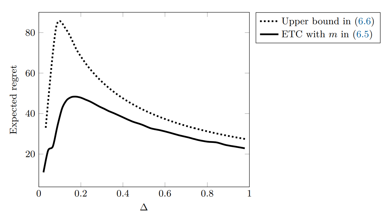
The figure above shoes the expected regret of ETC when playing a Gaussian Bandit with $k=2$ (two actions) for means $\mu_1 = 0$ and $\mu_2 = -\Delta$. The horizon is set to $n = 1000$ and the suboptimality gap $\Delta \in [0,1]$. Each data point is the average of $10^5$ simulations (that’s why there are no error bars). We can visually see that our constructed bound in Theorem $2.1$ is quite close.
This is the simplest and what my mentor calls the most “stupid” bandit algorithm but it’s still good to review for my own sake. In some ways, this parallels any betting game: when do we access the trade-off to commit to a strategy versus explore different strategies? What’s our EV (or in this case our constructed bound) for finding the optimal reward and sticking to such reward? Interesting thoughts I might explore later.