The More the Merrier: Multi-Player Bandit Information Asymmetry
For the sake of my own understanding (and sanity) I’m going to be summarizing a research paper that describes the mUCB-Interval algorithm.
This algorithm exists in the field of reinforcement learning and implements exploration-exploitation tradeoffs under different parameters compared to the ETC algorithm.
With two or more players, information asymmetry and, by extension, reward asymmetry occurs. We’ll be looking at how we tackle such imbalances and how we can still achieve desired sets.
Prerequisite Posts (if you care to follow along):
Source Material:
- Optimal Cooperative Multiplayer Learning Bandits with Noisy Rewards and No Communication
- Bandit Algorithms
Review of Regret and Reward
Although we looked at regret and rewards in Beware of Bandits, I’ll reiterate some terminology that the paper has in different notation.
Joint Action Consider a set of $M$ players $P_1, \dots P_n$ in which player $P_i$ has a set of $\mathcal{K}$ of $K_i$ arms to pick from. At each round, a player can pick an arm independently and simultaneously from other players from their set of $\mathcal{K}_i$. This joint action can be represented as a $M$-tuple of arms picked and denoted by $a = (a_1\dots a_M)$1. This generates $M$ iid. random rewards $X_a^i \in$[0,1] with $i \in$ [M] from a 1-subgaussian distribtuion $F_a$ with mean $\mu_a$.
Reward Asymmetry The idea that each player $P_i$ can only observe their rewards $X_i^a$ but are oblivious to all the other rewards is called reward asymmetry. Only after joint action is taken can they observe the actions of players. All players can determine a strategy and know the joint action space beforehand. However, during the learning process, they are not allowed to communicate.
Regret The optimal arm among all arm tuples is denoted as $\Delta _a = \mu*-\mu_a$ where $\mu*$ is the highest reward mean. The goal of these players is to pull the optimal arm as often as possible.
Let $a_t(i) \in (1, \dots K_i)$ be the arm chosen by player $i$ at time $t$ and deonte $a_t = (a_t(1), \dots, a_t(m))$. For the players to pull the optimal arm, the high-level strategy is to collectively identify the best set of arms $a$ corresponding to mean reward $\mu*$ given that they don’t know the distribution or the means $\mu_a$. To do this, they must learn by playing and exploring. The learning efficiency can be represented as expected regret,
\[\tag{1} R_t = \mathbb{E}\Bigl( T\mu* - \sum_{t=1}^T X_{a(t)}(t) \Bigr)\]$T$ is the number of learning instances and $X_{a(t)} (t)$ is the random reward if $a(t)$ is pulled. We let $\eta_a(t)$ be the number of times joint arm $a$ has been pulled up to but not including time $t$. Let $\hat{\mu_a^i}(\eta_a(t))$ to be the empirical mean of arm $a$ for player $i$ at time $t$ after $\eta_a(t)$ pulls the joint arm $a$. This empircal mean is indexed by the player since each get their own iid reward. In contrast, the regret $R_T$ is the same for each player because the reward for each joint arm has the same mean across all players 2. $\eta_a$ is not indexed by the player $i$ becuase each player contributes to the same joint action $a$ every round.
While each player will likely have different rewards, the rewards are iid and the regret will therefore be the same across all players. The paper uses the the suggested lower regret bound $O(logT)$ for the multi-player decentralized learning algorithm with the same regret order.
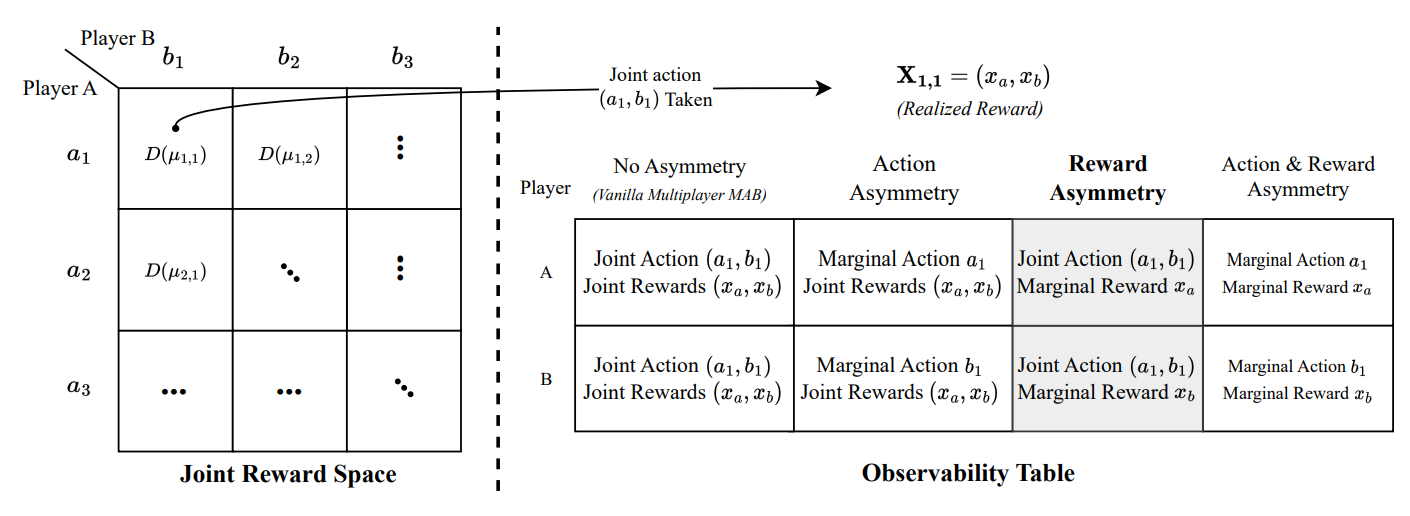
The left matrix is the joint action space of player a and b with each cell corresponding to a subgaussian reward distribution for some mean. The table on the right lists different types of information asymmetry. In this post, we focus on Reward Asymmetry in grey.
Main Results of mUCB-Intervals
The UCB Index
To maximize the cumulative rewards we define the *UCB index, also known as the Upper Confidence Bound for each joint action. The player’s objective is to pull the largest UCB index as often as possible. For each player $i$ we can define the UCB index as,
\[\tag{2} \eta^i_a(t) = \begin{cases} \infty & \text{if } \eta_a(t) = 0, \\ \hat{\eta_a^i}(\eta_a(t)) + \sqrt{\frac{2log(1/\delta}{\eta_a(t)}} & \text{otherwise.} \end{cases}\]Let $\epsilon_a(\dots)$ be the constant added to the empirical mean for arm $a$ in calculating the UCB index. This constant is the same for every player and therefore not indexed by $i$. Our algorithm introduced further in the post will be of length $2\epsilon_a(\dots)$. Because of this we add a tuning parameter $\gamma$ such that,
\[\tag{3} \epsilon(\eta_a, \delta, \gamma) := \gamma\sqrt{\frac{log(1\delta}{\eta_a}}\]Using Hoeffding’s bound for subgaussian variables3, the true mean $\mu_a$ is within the interval
\[\tag{4} I_a^i = (\hat{\mu_a^i} - \epsilon_a, \hat{\mu_a^i} + \epsilon_a)\]with high probability. We can use this confidence interval to create a set of arms that are likely to be optimal and to make this selection from this set. While this interval is different for each player $i$ given some joint action $a$ due to the empirical means $\hat{\mu_a^i}$ being different, $\epsilon_a)$ is not indexed by $i$.
Reward Asymmetry
To deal with information asymmetry, all players will maintain a desired set that contains the joint arms that are candidates for the optimal arm. Initially, $K^m$ joint actions are in this desired set; this desirability is predetermined by an arbitrary ordering.
A joint action is considered if it is the arm in the desired set that supposed to be pulled given the order that was agreed by all players. We denote this joint action in the desired action as $c$. If there is $l$ joint actions $c_1, \dots, c_l$ then the ordering of the desired set can be viewed by the following flow chart as,
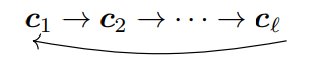
A joint arm is eliminated from the set if it does not fall within the UCB interval and is disjoint from another arm. Player $i$ effectively “communicates” this elimination to the other players by not pulling $c_t[i]$; the other players will also eliminate this arm from their desired set while maintaining order. Pulling a joint arm is not considered the same as removing a considered arm from a set.
The net flow can be visualized as,

Run-through Example
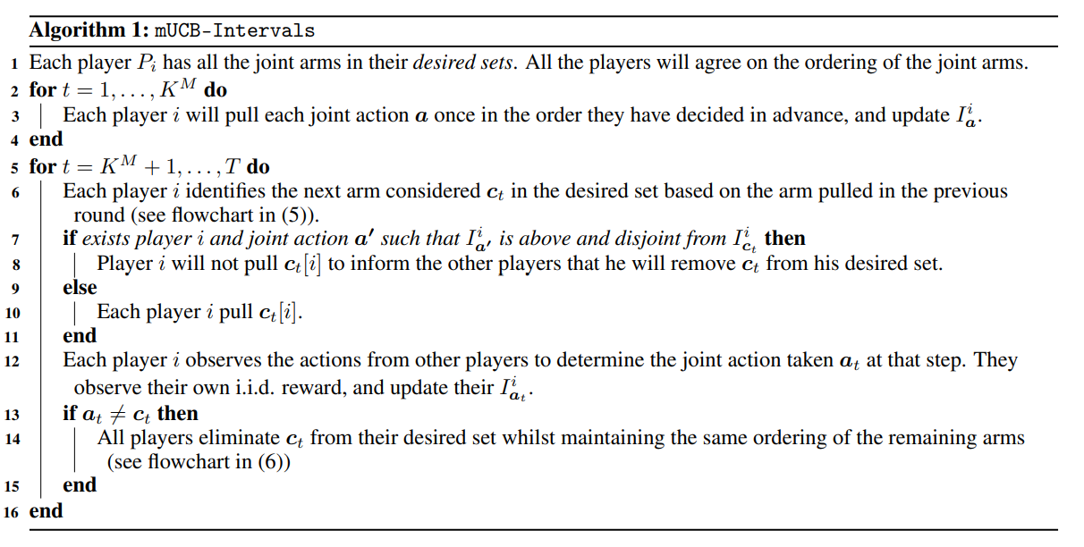
Consider a two-player setting where each player has two arms. We will represent each joint as as a matrix where each cell is the UCB interval defined in equation 4 (general visualization of the player environment can be seen in figure 1).
If the first and second row and column correspond to player 1 and player 2 respectively,
\[\begin{bmatrix} (-\infty, \infty) & (-\infty, \infty)\\ (-\infty, \infty) & (-\infty, \infty) \end{bmatrix}_1, \begin{bmatrix} (-\infty, \infty) & (-\infty, \infty)\\ (-\infty, \infty) & (-\infty, \infty) \end{bmatrix}_2\]Suppose the order of the joint action is $(1, 1), (1, 2), (2, 1), (2,2)$. Initially, all UCB intervals are infinite as each arm gets pulled at least once. Then after the joint action flow where $t = 4$, the matrices become,
\[\begin{bmatrix} (.2, .5) & (.3, .6)\\ (.55, .9) & (.65, .8) \end{bmatrix}_1, \begin{bmatrix} (.5, .7) & (.4, .7)\\ (.6, .9) & (.65, .8) \end{bmatrix}_2\]For round $t=5$, we consider $(1,1)$ again. But because the UCB interval is disjoint some arm, that being (2,1), player 1 knows with high probability that this arm is not optimal. To communicate this to player 2, player 1 will instead choose arm 2. Player 2 does not know player 1’s actions during the round, so it still considers (1,1); player 2 will choose 1. The joint action of these two players will be $(2, 1)$.
After choosing these arms, player 2 sees that arm 1 is suboptimal and now understands $(1,1)$ should be eliminated. The flow of the desired set now becomes $(1, 2), (2, 1), (2,2)$.
For round $t=6$, the next considered arm is $(1, 2)$ and the process repeats until we are left with the most optimal arm with the highest probability. In this case, this is $(2, 2)$.
Regret Bound Analysis
Theorem 1 For any choices of tuning parameter $\gamma > 0$, the gap dependent of algorithm mUCB-Intervals is
\[R_t = O\Bigl( \Bigl( \sum_{a \in \mathcal{A}} \frac{1}{\Delta_a} \Bigr) logT + MK^2)\]Theorem 2 For any choices of $gamma > 0$ the gap-independent regret bound of algorithm 1 is
\[R_T = O(\sqrt{KTlog(T)})\]Lemma 4 ith regret defined by equation $1$< the regret decomposition for player $i$ follows,
\[R_T^i = \sum_a \Delta_a\mathbb{E}(\eta_a(T))\]where $\eta_a(T)$ is the number of times the arm $a$ has been pulled up to round $T$.
Lemma 5 Under the event $G \cap G^{cross}_a$, the number of pulls of arm $a$ is at most $u_a$.4
The paper introduces a cooperative multiplayer bandit learning problem where players are only allowed to agree on a strategy beforehand but can not communicate during the learning process. Each player receives a noisy version of the reward that cannot be shared with other players. mUCB-Intervals based on upper and lower confidence bounds scaled by $\gamma$ can be used to select optimal actions despite asymmetry. This asymmetry can be ultimately removed and be used to derive an algorithm that gives asymptotically optimal regret.