Chapter 1: Market Microstructure in Practice
Like a gremlin searching for gold, sometimes I scour the internet for recommended textbooks and literature on stack exchange or reddit. It gives me perverse joy to hoard these little nuggets of knowledge in a text file on my computer, but alas, the list is too long for me in good conscious to keep stockpiling my spoils of online swashbuckling. I’ve begun the process of whittling my ‘tbr’ down with a gem called Market Microstructure in Practice by Lehalle and Laruelle.
Touted as a beginner friendly introduction to microstructure and its mechanisms, Market Microstructure in Practice primarily focuses on European market timelines and the evolution of Markets in Financial Instruments Directive (MiFID) regulation. Even if some microstructure design is not directly applicable to US counterparts, it’s still a very interesting read that has benefited my understanding.
I’ve decided to split this book into three separate posts, each dedicated to its own chapter. This series of blog posts aims to compress all my hand written notes and concepts introduced in Market Microstructure in Practice into an abridged notebook of sorts. I’ve outlined important concepts and some technical appendix insights that I found interesting and applicable while skipping some eulogies on the history of European markets and the birth of MiFID. Happy reading!
Below you can find a pdf of the textbook and my notes:

Liquidity in Question
Market Impact: If information symmetry occurs between buyers and sellers, sellers offer to sell at worse prices if the buyer is not stealthy enough.
Bid-ask spread: Is the distance between bid and ask price.
Slices: When an investor is seeking liquidity given a large order they will have to splice such order through venues. Optimal slicing is in reference to an optimal trading theory.
Decay: Decay of market impact serves to answer the question - if I consume liquidity on an asset at time $t$ how much time is needed for the price to revert?
Synchronization: Large buy orders can be obscured with sell orders if there are high levels of synchronization. Hence, market impact of a large order is the average over enough market configurations.
Price Formation Process (PFP): Buying or selling pressure that is not consistent with market participant consensus will only generate a temporary impact. The opposite is true for aligning motives of participants.
Microstructure of a Market: Defined as the way different traders share their responsibilities and roles.
How the Market Consumes Liquidity
Regulatory changes in 2005 have lead to new price formation processes that have shaped the market landscape. Now, HFTs act as market makers, a consequence of fragmentation within venues and products.
Because liquidity bridges need to be established to ensure orders are filled, arbitrageurs (HFTs) will take half the difference of the bid-ask spread and improve the level of information. Acting as information delegates, the price of HFTs adding to the fragmentation of markets is the increased flexibility of cross-trading between venues.
The Price Formation Process
Driven by information, the price formation process is a paradox of its own. Sharing information is adverse for an investor, yet it is essential to use information from other participants to make informed trades.
In the US this conundrum has manifested into regulations across asset classes. For fixed income and equities markets, the Centralized Limit Order Book (CLOB) or Request for Quotes (RFQ) is used. The differences are aggregated below.
RFQs:
- Bilateral
- Trader has fundamental information and dealer has information on flows (asymmetry of information)
- Trades are more exposed to opportunity cost while dealers are exposed to adverse selection cost
- Market makers widely use conditional orders RFQs to standardize refusal to trade.
- Stalled quotes are more present
CLOBs:
- Multilateral
- Participants are exposed to both opportunity cost and adverse selection cost depending on limit or market order
- Vanishing liquidity is more present
European Market Fragmentation
In the US, options are traded electronically or by using limit and market orders. This multilateral approach differs from European regulation which instead hinges on fragmentation of Central Counter Parties (CCPs) that make it virtually impossible to net-zero buy and sell the same option on different venues. Without normalization of CCPs, competition on the derivatives market is impossible.
When the Markets in Financial Instruments Directive (MiFID) was created in 2007, the European Union sought to change equities markets by liberalizing trading venues and creating a ‘best execution policy’. However, the application of the directive was surprising - liberalization created only a small number of alternative trading venues (Chi-X, Turquoise, BATS Europe, NASDAQ-OMX) which created high levels of competition - splitting markets into niches.
The ‘best execution policy’ was a matter of offering consolidated access to liquidity by both passive and aggressive orders through Broker Crossing Networks (BCNs), Smart Order Routers (SORs), and others.
The Importance of Market Microstructure
At its core, market microstructure generates the price formation process. This process is the “heart of capitalism” that balances supply and demand through the context of information. The more information available to trades, the better the PFP becomes. Conversely, information leakage and front running can create negative price impacts.
The general consensus of the PFP is that it encompasses each trade occurring in the market combined with “fair price” of the listed asset. This can be split into two phases,
- Phase 1 deals with the impact of price given movement with buys and sellers, liquidity consumers and takers. This is coined the immediate price impact.
- Phase 2 consists of liquidity returns in concordance with spread and fair price. The decay of impact from these liquidity behaviors is also known as the resilience of the limit orderbook.
Fluctuations of Market Shares: A First Look at Liquidity
Levels of Market Fragmentation
- Market operators
- Trading Venues
- Orderbooks
- Orders themselves
- Technology
Let $M$ be the number of transactions that took place from $t_1$ to $t_2$ over $N$ venues. If $l$ is each individual trade then the price for each trade is $P_l$ for volume $V_l$ at time $\tau_l$. $\delta_1=n$ is the number of trades occurring on individual venue $n$ (where this value is 1 in the indicator function). The market share of venue $n$ on stock $k$ is given as $$\begin{align} \mathcal{M}^k(n) = \frac{\sum_{t_1 \leq \tau^k_l \leq t_2}P^k_lV^k_l \times \mathbb{1}_n(\delta^k_l)}{\sum_{t_1 \leq \tau^k_l \leq t_2}P^k_lV^k_l} \end{align}$$
When price of stock $k$ is relatively constant such that $\forall l: P^k_l \approx P$, we can reformulate market share as
\[\begin{align} \mathcal{M}^k(n) \approx \frac{\sum_{t_1 \leq \tau^k_l \leq t_2}V^k_l \times \mathbb{1}_n(\delta^k_l)}{\sum_{t_1 \leq \tau^k_l \leq t_2}V^k_l} \end{align}\]To compute the market share per trade we can divide over total trades $T$, $$\begin{align} \mathcal{M}^k_T(n) \approx \frac{\sum_{1 \leq l \leq T} \mathbb{1}_n(\delta^k_l)}{T} \end{align}$$
If we understand that fixing auctions change market share (more on this later), we take into account the monopoly the venue has over said auction. If venue $\mathcal{T_n}$ has an average market share of $m(n)$ during a fixing auction with weight $p$ of overall venue activity and average daily turnover $\mathbb{T} = \sum_{1 \leq l \leq T}P^k_lV^k_l$, then the average market share of a fixing auction is
\[\begin{align} \mathcal{M}(n \text{; ex-fixing}) \approx \frac{(1-m(n))p \times \mathcal{M}(n)\mathbb{T}}{(1-p)\mathbb{T}} \\ \approx \frac{1-m(n)p}{1-p} \times \mathcal{M}(n \text{; all included}) \end{align}\]Market Weights
When computing the market share of multiple stocks we look at weighting each stock by daily turnover. We can represent our market share equation as,
Weighting by market share of of stock $k$ according to weight $w_k$ in a given index $J$ is given by
\[\begin{align} \mathcal{M}^{J}(n) = \sum_{k \in J}w_k \times \mathcal{M}^k(n) \end{align}\]The index is often proportional to the market capitalization of the stock and is not usually interpreted with daily turnover.
Measuring Metric Adequacy
Analyze the positioning and revenue of each trading venue.
- The market share (all included) can be important even in terms of venue.
*Measuring the probability when a trade occurs for security $k$ is on venue *$\mathcal{T}(n)$.
- Instead of summing fixing auctions with the continuous ones, use market share during the fixing auctions and ex-fixing as separate indicators.
Measuring the probability that, when a unit of currency (euro, dollar) is traded on security k, it is on trading venue $\mathcal{T}(n)$.
- The classical market share value $\mathcal{M}^{k}(n)$ is the best given we want to make one measurement during the fixing auction and another for intraday.
Appendix A.8. Estimation of Proportion and its Confidence Intervals
In microstructure we have to estimate proportions and probabilities using a binomial distribution (collection of bernoulli trials). To estimate the success the probability of success we use the empirical mean of the trials where $\hat{p} = \frac{1}{n}\sum^n_{k=1}X_k$. This unbiased estimator ($\mathbb{E}[\hat{p}]=p$) and variance $Var(\hat{p}) = \frac{p(1-p)}{n}$.
Given SLLN (Strong Law of Large Numbers) the estimation converges to $p$ as $n \to \infty$. By the central limit theorem (CLT), the empirical mean converges to a normal distribution. With a level of $1-\alpha$ we can approximate a confidence interval of $p$ such that,
\[\begin{align} \hat{p} \pm z_{1-\alpha/2}\sqrt{\frac{\hat{p}(1-\hat{p})}{n}} \end{align}\]where $z_{1-\alpha / 2}$ is the $1-\alpha / 2$ percentile of a standard normal distribution.
First Attempts of Fragmentation
A simple statistic to follow the fragmentation of European markets is the market share of the historical markets on each main index of each country. Given the increased competition and decreased market share, MiFID’s foray into fragmentation:
- Halted the monopolistic position of historical exchanges
- Promoted pan-European microstructure
- Created LSE Group
- Merged Chi-X and BATS
These niche markets offer two specific mixes of liquidity:
- Natural liquidity: comes directly from investors buying and selling for medium to long-term held positions.
- Opportunistic liquidity: which are offered by HFTs and market makers.
These types of liquidity allow for investors to create their own mix of liquidity and segmenting needs, proliferating the creations of mid-point dark pools, buy-side only pools, size-priority books, and random-auctions. Increasing the number of liquidity sources (like increasing the degrees of freedom) increases the complexity of allocation and cost of providing an aggregate view.
MiFID's cause of fragmentation increased complexity with three different components:
- Best execution
- Three statuses for trading venues
- Pre-trade transparency rules
Best Execution
The European Commission does not provide a consolidated tape or route orders to be filled elsewhere for European markets. This diversity of clearing and settlement channels brings cause to potential inversion of best prices. Combined with intermediary best execution policy of routing procedures, it proliferated the creation of a two layered competition model designed to put pressure on intermediaries and venues to offer the best mix of liquidity and improving the PFP.
Trading Venue States
MiFID constrained executions on four markets:
- Regular markets (RM): host a matching engine that executes orders on a public order book. These markets are responsible for integrity of PFP.
- Multi-lateral Trading Facilities (MTF)s: transactions are matching in a engine on public orderbooks more often pegged to the state of orderbooks in RMs.
- Systematic Internalizes (SIs): executes orders based on bilateral agreements between counterparts (one of them being a market maker)
- Over the counter
Pre-trade Transparency
MiFID allowed for the disclosure of the orderbooks state to traders, also known as pre-trade transparency. This demand comes from the need for information that is disclosed to decision-makers; the more rational participant actions become from this information the more efficient the PFP will be - increasing a principle demand for pre-trade transparency.
A price can be formed by executing a liquidity demanding order against a resting order only if the state of the orderbook is disclosed to all market participants. Some exceptions exist:
- A large in scale waiver can rest in orderbooks without transparency
- Order management facility waivers exist to protect trades from information leaks
- Negotiated trade waivers that are priced within VWS
- Reference price waivers allow hidden orders of any size provided they do not form a price via confrontation of offer and demand. They can be traded at a fixed price - if this happens the transparency is delegated to the reference venue (dark pools).
Post-trade Transparency
Another obligation of the PFP process is post-trade transparency. This trade dissemination ensures investors and traders make rational choices and have the proper level of information on the last price at which the participant agreed to trade upon. But again, this transparency comes with a cost - more information increases rational decisions yet investors are worried about information leakage that shorten investment horizons and profit.
Entropy of Market Microstructure
Applying statistical thermodynamics, it’s worth noting that measuring the dispersion of matter or the level of randomness is called entropy. If the consolidated market is considered a system, “order” is all orders on one venue wile “disorder” increases with fragmentation (A.1.).
The formula for entropy is used to define the Fragmentation Efficiency Index (FEI) which models the microstructure of $N$ trading venues (assuming in relaxed state) where liquidity could find its way to any venue at the same cost. An ideal or minimal fragmentation is $1/N$.
$$\begin{align} \text{Entropy } = -\sum^N_{n=1}\mathcal{M}_n \log \mathcal{M}_n \end{align}$$
- When only one liquidity pool is available the entropy of the system is zero
- When all liquidity is concentrated in one pool the entropy for the system is zero
- When there is equal allocation of liquidity in each pool $H=\log N$.
The FEI of a distribution of liquidity $q_1, \dots q_n$ for $N$ pools is the ratio of entropy $H(q_1, \dots q_n)$ divided by the possible entropy over $N$ pools.
$$\begin{align} \mathcal{F} = \frac{H(q_1\dots q_n)}{\log N} = \frac{-\sum_{1\leq n\leq N}q_n \log q_n}{\log N} \end{align}$$
The FEI measures the efficiency of the repartitions across liquidity pools compared to a uniform one. The closer to zero, the more concentrated liquidity, the more inefficient the microstructure is. When closer to one the fragmentation is efficient - a trader does not need to pay much attention to the smart routing given all sources are valued equivalently.
HFT Activity Outside of Visible Pools
The rise of HFTs in conjunction of the global decrease of European liquidity dulled the confidence of the price formation process. In light of the Flash Crash, many were hooked on the idea that HFTs earned a part of the bid-ask spread by taking profit from other participants.
Fragmentation created different pools of liquidity to host specific investors. MTFs offered second hand liquidity where historical pools offered more first hand liquidity; this, coupled with increased fix cost from fragmentation pushed demand on pools marketed as wholely first hand liquidity. This caused the birth of Broker Crossing Networks (BCNs).
Catching Up Main Indexes
The evolution of market share for 600 of the most liquid European stocks can be seen in figure 1. We see that in the mid-2009s large caps were much more fragmented - by 2012 the difference between mid and large caps is marginal.
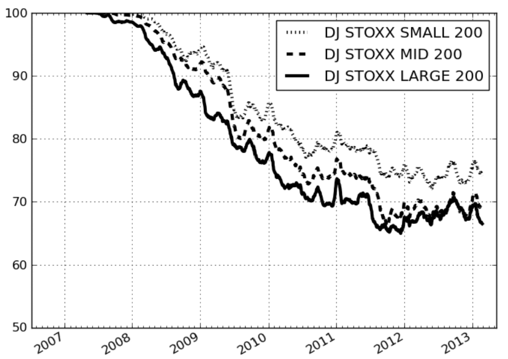
The differences of the three segments can be explained by
- Liquidity providing microstructure: Providing liquidity on the ask side without officially being a market making meant borrowing shares. Borrowing costs decrease with the number of shares available, hence asymmetry for the provision of liquidity that caused fragmentation among caps.
- Unbalanced inventories: For HFTs and market makers to buy and sell correlated instruments hedging using futures usually had a smaller bid-ask spread. This meant that it was easier to sustain unbalanced inventories on large market caps given their underlying feature on future contracts.
These two reason allowed for liquidity arbitrageurs to accept inventory risk on large market caps, increasing fragmentation levels for cap levels.
Measuring Liquidity Discrepancies
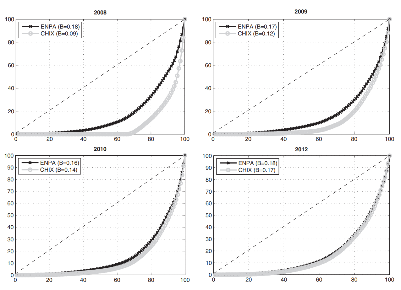
The Gini-coefficient and the Kolmogorov-Smirnov test allows us to measure repatriations of the different types of actors in the market (A.9.).
The Gini coefficient is the measure of degree of inequality of income distribution in a given society. Zero represents total equality while one represents total inequality.
In statistics the Kolmogorov-Smirnov test is used to determine if a sample follows a known probability distributution given by a continuous distribution function. The empirical distribution $F_n$ for $n$ iid. observations $X_k$, $1 \leq k \leq n$ is defined as,
\[\begin{align} \mathcal{F}_n = \frac{1}{n}\sum^n_{k=1}\delta_{\lbrace X_k \leq x\rbrace}. \end{align}\]$\delta_{\lbrace X_k \leq x\rbrace}$ is the indicator function that equals one if $X_k \leq x$ and zero otherwise. The Kolmogorov–Smirnov statistic for a given cumulative distribution function $F(x)$ is,
\[\begin{align} \mathcal{D}_n = \sup |F_n(x) - F(x)| \end{align}\]Given the Glivenko–Cantelli theorem the sample comes from distribution $F(x)$ then $D_n$ converges to $0$ almost surely.
$$\begin{align} H_0: \sqrt{n}D_n \to_{n \to \infty}^{\text{law}} K \end{align}$$ K is the random variable with the Kolmogorov distribution. The null hypothesis is rejected at level $\alpha$ if, $$\begin{align} \sqrt{n}D_n > k_{1-\alpha} \end{align}$$
Plotting the evolution of distributions between 2008 and 2012 for market share of SBF 120 on Euronext Paris and Chi-X and their associated Gini index we note Chi-X’s increase in market share Conducting a Kolmogorov–Smirnov test checks if the market shares of the venues have the same distribution. By the given data the null hypothesis is rejected in 2008 and 2009 but accepted in 2012 and 2012.
SOR (Smart Order Routing) and the European PFP
Routing Orders in a Fragmented Market
Large orders are spliced with consideration on market impact and market risk given adverse moves in prices. Risk Aversion is used as a parameter to measure optimal trading schedules. Given market risk and impact are not linear and volume and volatility experience intraday variation, optimizing leads to non-linear trading curves.
Focusing on the best way to split the quantity of a large trade among venues will be optimal if
- It obtains a price better than or equal to the asked price.
- It finishes the order as soon as possible.
The best way allocate orders is to not consume a whole limit on a price in the main destination if volume is available in alternative venues. A SOR completes this optimization as an agnostic device - it takes a limit or market order and splits it with advanced knowledge of the state of liquidity on the destinations that are ready to trade.
Aggregating Liquidity to Minimize Impact of Order
A consequence of electronic trading is the increase of deals with current trading sizes conditioned on the size of passive orders. The average trading size of orders have decreased, signaling an increase in market fragmentation and more passive orders spread over more destinations.
Duplicate Liquidity
HFTs and market makers are simultaneously at bid and asks of a security on several destinations. They agree to take on market risk and are rewarded with the fraction of the spread - but when liquidity is posted on the same side of the orderbook on different venues, as soon as one is executed, the other orders are cancelled. This leads to “duplicate” quantities in the orderbook, undermining pre-trade transparency.
SORs dynamically split an order across venues to take into account historical performance of their executions. An order with large variance will be minimized by a rational SOR
Optimal Tick Size
Tick size defines the price grid on which a limit order must lie. Depending on the market it can be applicable to price and liquidity or dependent on price range and quotation group of the stock.
Tick sizes set the discreteness of traded prices. Larger tick sizes with a constant spread will base volatility as a function of tick size - uncertainty on the text traded price in context depends on sizing of ticks.
Measuring Spread and Volatility based on Tick Size
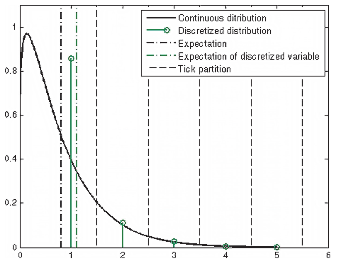
The Harris Model serves to understand the underlying continuous spread discretized by tick.
Some caveats are highlighted below:
- Turnover $T_j$: Determinant of spread given proxy for liquidity
- Volatility $\sigma_{j, d}$: Determinant of spread because of extra risk taken by limit order traders when providing liquidity.
- Price $P_{j, d}$: Not a determinant of relative spread because providers are indifferent about nominal price of supplied liquidity.
- $\tilde{\mathcal{f}}_{s, \theta}$: density of underlying continuous spread.
- $\psi_{j, t} = \frac{\text{Ask - Bid}_{j, t}}{\text{Tick}_d}$: This is the observed spread in ticks for stock $j$ on the $t$th trade on day $d$.
$$\begin{align} \psi_{j, t} = \phi(\tilde{\psi_{j, t}})\end{align} \\ \mathbb{E}[\tilde{\psi_{j, t}} | T_j, \sigma_{j, d}] = g(T_j, \sigma_{j, d}) \times \frac{P_{j, d}}{\text{tick}_{j, d}}$$
Seen in figure 3, the model is consistent with the discreteness of observed spread and will quantify the increase of expected spread from continuous to discrete distribution. The discretized distribution $\mathcal{f}_{s, \theta}$ is made up of Dirac densities (used to model spike functions).
If we reformulate the expectation of spread measured in tick size conditioned on turnover and volatility as a log linear relationship we use the maximum log likelihood to attain the maximum likelihood estimator $\hat{\lambda} = arg\max_\lambda l(\lambda)$:
\[\begin{align}\mathbb{E}[\tilde{\psi_{j, t}} | T_j, \sigma_{j, d}] = \alpha \times T^\beta_j \times \sigma^\gamma_{j, d} \times\frac{P_{j, d}}{\text{tick}_{j, d}}\end{align}\]$$\begin{align}l(\alpha, \beta, \gamma, \theta) = \sum_{j, d, k} \ln (f_{\mathbb{E}[\tilde{\psi_{j, t}} | T_j, \sigma_{j, d}], \theta}(k) \times N(f, d, k))\end{align}$$
For a numerical example of the harris model, we can use the 60 most liquid stocks on the FTSE, an underlying spread gamma distribution, and maximize likelihood to estimate the parameters.
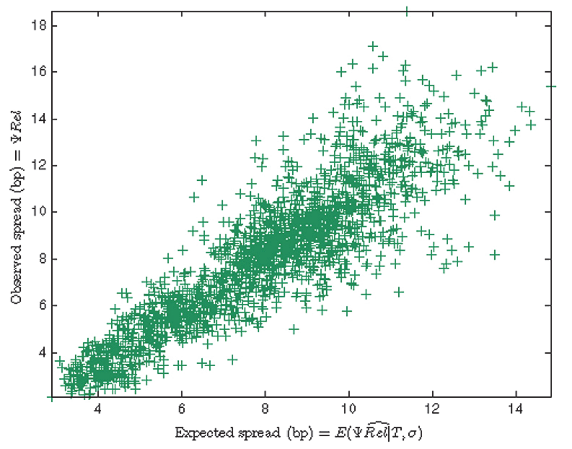
The pseudo R-Squared value is 0.8.
How Tick Size Affects Market Quality
- Decreasing te tick size lowers spreads when tick size is a constraint
Tick sizes will eventually act as a minimal bound for the bid-ask spread acting as a constraint in two ways:
- Binding probability: Percentage of trades or duration of quotes with a spread equal to one tick.
- Spread leeway: The spread expressed as tick units minus one.
Does increasing the tick size increase the cost for a liquidity taker?
A smaller tick size will split limit orders over more price points - this causes less quoted size at each limit price. Queue jumping commences with small upticks in price to gain queue priority. Quoted sizes on the best limits are therefore much smaller with a small tick size. Furthermore, the mechanical consequences of having more price points to spread your order on is the incentive to conceal full sizes of orders. Queue jumping makes participants less inclined to show size of orders to void being front run.
Cumulative Depth and Order Exposure Incentive
Dissecting execution cost can be achieved through comparing post and pre event costs for any volume to tell which orderbook is sounder. This approach takes into account hidden liquidity.
Some other models were reviewed:
- Bacidore 2003: Showed for any given size the expected cost of a marketable order was lower after decimalization
- Found that at orderbook at anytime with and without conditional of the occurrence of a trade. This gave insight ont he resiliency of the orderbook and its ability to replenish queues with liquidity after consumer traffic.
- Found that liquidity was worse after tick size change for deeper limits.
- Goldstein, Kavajecz 2000: They found that the publicly available orderbook was less deep after decimalization and the cost of a virtual large trade for frequently traded stocks was greater.
- Found that the cost for small-sized orders decreased but there was no improvement for trading a large size on a high price frequently traded stock. This gives us insight on order exposure incentive.
In summary, tick size reduction harms the liquidity by increasing costs.
Unlike European markets, US’s large tick sizes have larger spreads so that someone able to undercut a limit order with small price concessions will be able to make the market, hence earning a large spread rent. Given maker-taker fees (rebate to provider and fees on consumer) are expressed in dollar per share - not the relative trade value traded - rebates are much higher on lower priced stocks. This is a sound incentive to provide liquidity for low priced stocks which helps competition for liquidity provision with small price improvement.
Notes on Queue Jumping
With huge volume at the first limit and a spread equal to tick size, fairly fast execution will need to be in the form of a market order. Providers will have to be careful about queues given the timing for a limit buy. Small tick sizes can achieve fast execution through price improvement – shifting it’s focus from queueing problems to limit price issues.
Can We see in the Dark?
Dark pools in Europe were created as a result of MiFID to increase competition and consumer protection in investment services.
Dark pool is the generic name for an exchange that does not publicly announce available liquidity. Almost like a spin off of manual telephone trading, dark pools make the PFP much more complex.
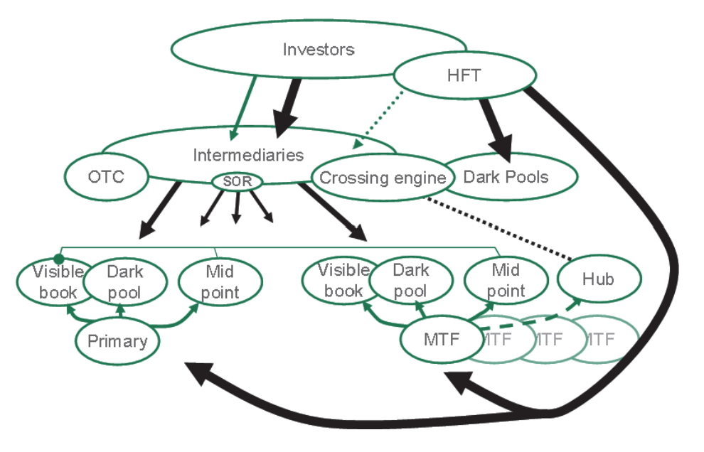
Mechanisms of Dark Pools
The main types of dark pools are listed below:
- Crossing Networks: Pools of liquidity that cross buy and sell orders for the same stock using mid-prices derived from the primary market. WHen we talk about dark pools this is the general pool we refer to.
- Internalization Pools: Pools where a Broker internalizes its own flow.
- Electronic Market-Makers: These pools do not cross orders with other client orders but with the operators flow. Electronic market-makers immediately reject or accept orders.
- Exchange-based pools: This is dark liquidity hidden on lit pools. These orders are executed when the counterpart is larger that a certain threshold.
- Dark Aggregators: This provides to all dark pools simultaneously to create a single point of fragmented liquidity. They receive an order and split it across various pools.
- Size Discovery Pools: These are large block dark pools that host natural liquidity (from institutional investors only).
Distinct orderbooks (MiFID regulated):
- Integrated book: Accepts all visible orders and hidden orders that are “large in scale” (LIS).
- Dark or mid-point book: Accepts hidden orders smaller than the LIS metric and matches only at the mid-point of the primary best bid and offer.
Hence order routing depends on order size - LIS orders participate in PFP while smaller orders are matched at mid-point.
Dark Pool Price Discovery
Prices can not be created in dark pools and only serve as liquidity reservoirs. Transactions are made at mid-price of the primary market and do not directly (but they do indirectly) participate in PFP.
How do we understand the role of dark pools in the price formation process?
- What are the types and quality of information present in crossing networks?
- What are factors that motivate someone to choose a lit or dark pool?
- What is the relationship between dark vs. lit pool activity?
Based on Buti 2010:
- Dark pool activity is concentrated in liquid stocks.
- Activity is higher in days with high share volume, depth, and lower intraday volatility.
- Activity is lower in days with large order imbalances relative to share volume.
- Activity is associated with short-term overreaction.
Main Characteristics of Dark Liquidity
Based on Rosenblatt Securities 2012,
- Execution sizes decrease compared with preceding years.
- There is no clear relationship between market share and volatility.
- Broker-dealer pools dominate exchange-based dark pools.
- There was a modest dark pool market share growth in the US during 2012.
Reasons to trade in dark pools:
- Fear of revealing trading intentions. Institutional traders want to keep their orders secret and allow them to to be crossed against other institutions
- Enable investors to be more aggressive without paying the whole spread (trading at mid-point)
Hypothesis: liquidity is mainly driven by the appeal of earning part of the spread.
To set out to prove the hypothesis, we looked at data consisting of VWAS, volatility, and turnover traded in the dark. For a single stock the VWAS and volatility was split into ten deciles and summed over the turnover traded according to said deciles. Summing all the turnovers on all stocks, we can view the joint distribution of VWAS, dark pool turnover, and the distribution of dark turnover, conditional on VWAS.
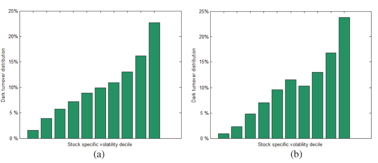
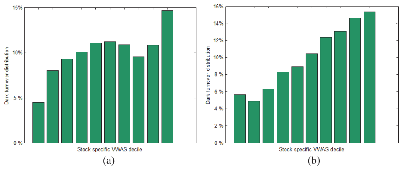
Given figure 6 and 7, either the spread or the volatility is related to the volume traded in dark pools. The link between volume and volatility being stronger that spread and volatility implies we must moderate the conclusions we draw from a sole volume-volatility correspondence.
If we focused on dark pool market share and volatility or spread we can see volatility is not the strongest incentive for investors to use dark pools. Figure 8 illustrates this by breaking the volatility and turnover for a single stock into deciles and dividing the former over the latter, repeating the computation over all stocks of an index.
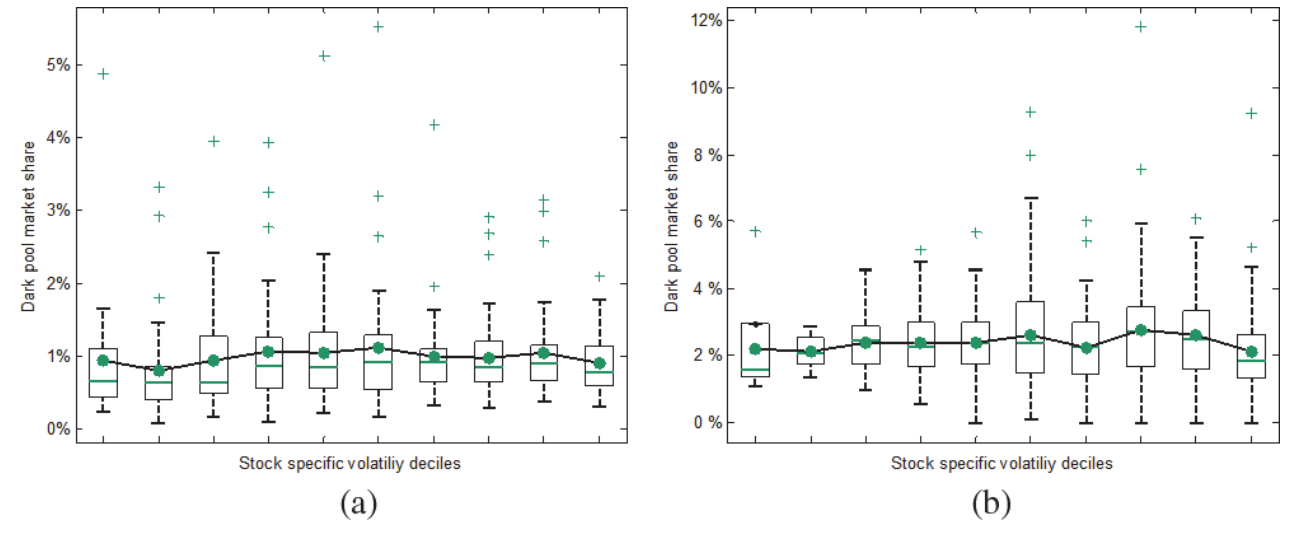
In contrast, relationships between spread are high. Indeed, the median dark pool market share is three times as high in the last decile of the spread as in the first decile - the higher the spread the easier it will be to find liquidity in dark pools.
This makes sense given the fact that when an investor really needs to trade a stock fast that has a high spread they will look at dark pools before sending a market order. This is because earning a half spread when the spread is consequential is beneficial. Dark pools are also used for reducing market impact if lit pools have lesser liquidity.
Chapter 1 notes are complete! There was quite a bit of timeline information on MiFID which I chose to omit - the curious reader can find more about that at the end of the ‘Introduction’ section. Appendix material I omitted included A.10 Simple Linear Regression Model and A.3 Natural Fragmentation of Market Microstructure.
Chapter 2 and 3 consist of understanding the stakes of fragmentation and the optimal organizations for trading. Those will be posted soon, but in the mean time feel free to take a look at my notes or the textbook.