Chapter 3: Market Microstructure in Practice

At last, here we are! The penultimate chapter of Market Microstructure in Practice by Lehalle and Laruelle focuses on optimal organization for optimal trading. We’ll look at fragmentation, market impact given the PFP, price anticipation and permanent market impact, price formation under conditioning, and orderbook dynamics.

Happy reading!

Below you can find a pdf of the textbook and my notes:

Organizing a Trading Structure to Answer a Fragmented Landscape

Main Inputs of Trading Tools
Large asset managers concentrate on tasks of mounting and unwinding positions to dealing desks, which takes care of:

The relationships with intermediaries.
Measuring trading costs and comparing broker performances thanks to Transaction Cost Analysis (TCA).
Choosing benchmark to target (VWAP, TWAP, Implementation shortfall, Target Close) according to investment style that generated the trade.

Dealing desks demand accuracy. Exchanges provide services around best execution (SOR), vendors provide better performance measurements and comparison features.

Market Data

Real time market data feeds are the eyes of a trading algorithm. Consolidated data is needed and the source should be easily disaggregated to know which trading venue is currently offering this price.

Market data contains:

Market trades, described by price, quantity, and timestamp
Limit orderbooks (bid-ask prices, quantities available, number of different market participants contributing at each price level), or sequences of modifications of the orderbook

Data is enriched with analysis with bid-ask spread, qualifying the observed market trades, intraday volatility, efficient bid-ask spread, or estimates of hidden quantities in the book.

Connection to Venues Algorithms need to be connected to exchanges. Connections are not natively synchronized with the market data and are two-way:

One to send messages to the trading venue: Creation of a new order, cancellation, or modification of another order.
The other to receive messages from the trading venue about the orders of the trading algorithm. Acknowledgements of messages sent by the algo, rejections, cancellations, partial fills, ect.

Incoming messages can be used as information probes. In dark pools, given no pre-trade transparency, orders sent by algos can be used as probes coming back with information about the state of the orderbook. When a dark buy order is filled at a given price, the orderbook of the dark pool contains resting sell quantities at the price or better.

Historical Data Optimal trading relies on intraday risk control and usual rhythms and behaviors of market features that are captured by models whose parameters are estimated by stock-by-stock or sector-by-sector basis. Historical data is needed and should contain:

Market Data (tick-by-tick or order-by-order)
Analytics that have been computed in real time
Recordings of the messages sent and received by the algorithms of the firm
Context-related information lik news, corporate events, activation of circuit breakers, outages of trading venues, ect.

Models A model is based off of three components:

The Formula: Takes in input parameters and variables. Parameters can be estimated once per day and sorted, the variables are known in real time and have to be plugged in the formula on the fly.
Estimation: A mathematical procedure taking as input historical data on a given universe and a given horizon and computing estimated values of the parameters of the model.
The accuracy computation: A mathematical procedure to quantify the quality of the model and its parameters according to the immediate past or in real time.

Components of a Trading Algorithm
Trading algos can be launched by a external user or by other algorithms. The different components are:

The execution parameters: Defines the execution conditions that apply to the algorithm
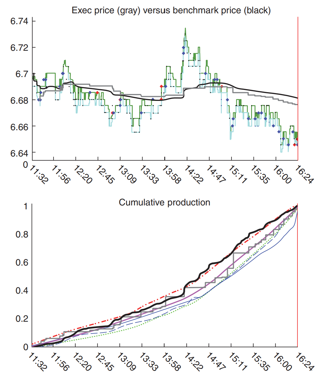
The risk control layer: In charge of computing reasonable maximum and minimum trading rates to target during the trading: This is called the trading curve. The layer uses models and expected market contexts to produce minimum nd maximum trading envelopes to follow in order to make the balance between two main sources of risk: market impact and market risk.
Trading robots or liquidity-seeking tactics: Like SOR, these are more sophisticated opportunistic tactics dedicated to navigate inside the trading envelope defined by the risk control layer. These robots have to take into account the immediate state of the liquidity to extract as much value as possible from venues.

The two layers, risk control and tactics, communicate through the risk control layer by sending messages to tactics to assign them short-term goals.

In figure 1 the trajectory of a trading algo is shown with the trading envelope and the real trajectory of the algo.

exec_price — Figure 1. The price and the obtained trades (dots); below: The cumulated traded quantity by the algo (grey), by the market (dark), the envelope can be seen in dot-dash lines

Main Outputs of an Automated Trading System

Pre-trade Analytics: The historical data, the models, and their parameters have to be used to provide decision support before the effective launch of a trading algorithm.

Pre-trade analytics are useful for the portfolios to check consistency of a portfolio and generate automated directives to speed up lines and slow down other according to pre-computation of the balance between expected market risk and expected market impact.

Typical pre-trade analysis includes:

Estimation and comparison of expected trading cost components (spread, traded volume, quantities on the books)
Expected trading profiles
Expected context (news, volatility levels)
Breakdown by sector, currency, country, ect.

Monitoring Indicators
Once an algo has been launched it has to be monitored by traders. Traders usually monitored several hundreds of working algos - indicators allow traders to build diagnoses of the algos on the fly.

Performance Indicators
A specific subset of monitoring indicators are direct measures of what the performance would be if trading should stop now and others include estimates of the performance when it will end, seen from now.

Typical performance indicators come from the decomposition of the average price of the trading algorithm according to different effects.

AVG price = Immediate Price + Market Moves + Market Impact.

On a benchmark-by-benchmark bases, such a decomposition can be refined towards

AVG Price = Immediate Price + Planned Price + Unexpected Market Moves + Trading Efficiency + Market Impact.

Planned price is what the risk control part of the trading algo expected on average. Trading efficiency rates the success of the liquidity-seeking tactics used by the trading algo.

Where to Produce Real Time Indicators
Algorithms themselves produce the indicators to publish. Indicator publishers are compatible with the fact that trading algos can be modeled as stateless agents and should have introspection capabilities; publishing views on their own state in real time to share with final users of companion als is an important component of modern trading algos.

Post Trade Analysis
Three components should be compatible:

For the spread:

The pre-trade analysis gives an expected average value.
The monitoring gives the current value, the updated expected average value, and the likelihood of the current value with respect to what happened so far. It gives the ability to quantify the relationship between the current trading performances and the trajectory of the spread.
The post-trade analysis gives an assessment of the value of the spread during the trading and its influence on trading performance.

Transaction Cost Analysis (TCA)
TCA is used by different algo providers to compare the efficiency of their trading over several weeks.

Post-trade analysis (day to day) aims to understand what happened because of the market context.

Requires fine grained analysis of market behavior. TCA aims to to explain the part of performance comes from the design o the trading algorithms.
Requires on averaging huge datasets to cancel most of market effects.

TCA associates a given trading algo with a give market context of trading style so that the user of the algo will send flow to the proper algo provider given market conditions. TCA involves breakdowns according to the characteristics of the market (volatility, jumps, liquidity, occurrence of news, etc.).

Liquidity is important to consider given it is useless to compare the efficient of an execution on a very liquid stock with one illiquid stock.

Typical indicators used to quantify liquidity are:

bid-ask spread
tick size in basis points
quantity on the books
daily turnover
average trade size
free float
trading rate

Market Impact Measurements: Understanding the PFP from the Viewpoint of One Investor

Factors that drive market impact:

liquidity of traded stock
quantity which is executed relative tot he overall quantity traded by other participants
aggressiveness of the trading algorithm
duration of the execution

Trade timing describes how an order is being traded compared to what happens in the market. Timing tells you if you are a trend follower or mean reverter. Timing tells you if the way you trade makes you visible to HFT eyes.

Market Impact Over the Trading Period
The benefit of intraday analysis of market impact is to quantify the changes in the market impact as an order is being executed and the dilution of this impact after the end of an execution.

The difference between the price at any given time and the arrival price is a good and frequently used measure of market impact.

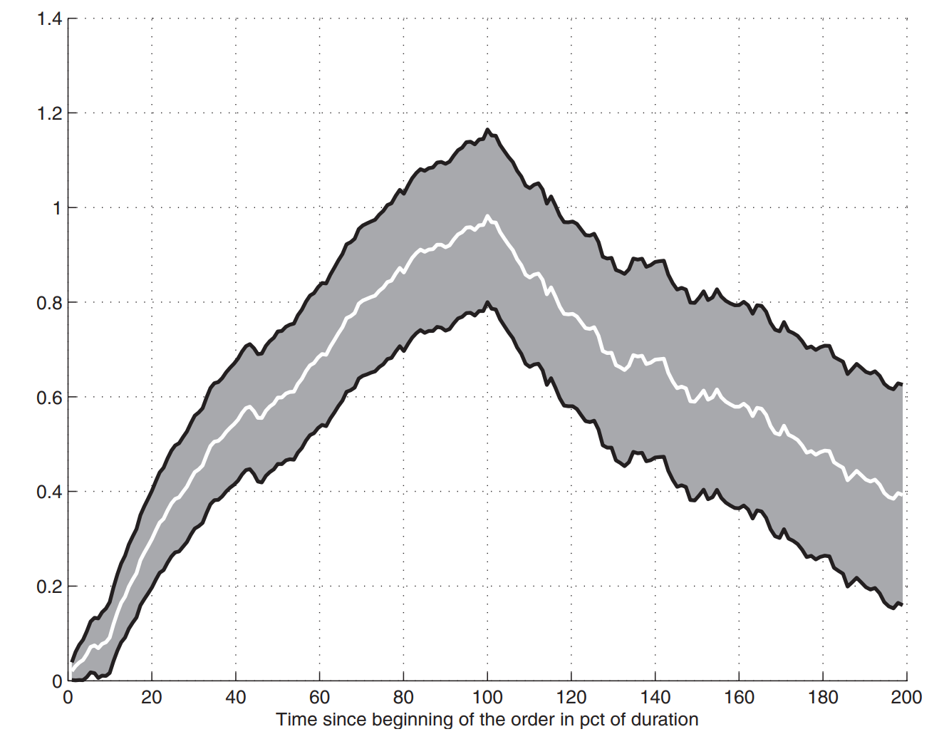
timing — Figure 2. Intraday market impact in spreads

Figure 2 shows the price of a stock while an order is being executed. If the returns of the stock is in the perspective of a buy order, prices above 0 means the investor will pay more to purchase a share or will be paid less to sell vs the beginning of execution. The grey bands represent the 95% confidence interval;the white line is the average. At 0 to 100 the impact curve is concave. At 100 to 200 shows the returns revert back.

Market impact may depend on several parameters.

Stock specific characteristics:

liquidity of stock
volatility
spread size

Order-specific characteristics:

aggressiveness of execution
quantity to execute
expected duration

Structure of the Dependency Between Market Impact and Parameters
Period Liquidity Ratio (PLR): participation rate

In figure 3 we plot the market impact for different values of the participation rate.

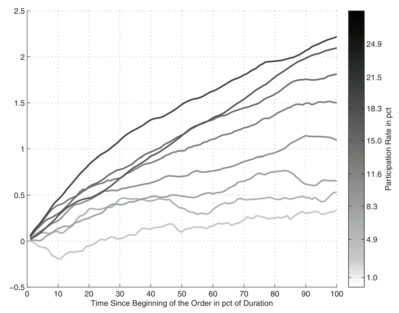
It can be seen that market impact curves get steeper as the participation rate increases.

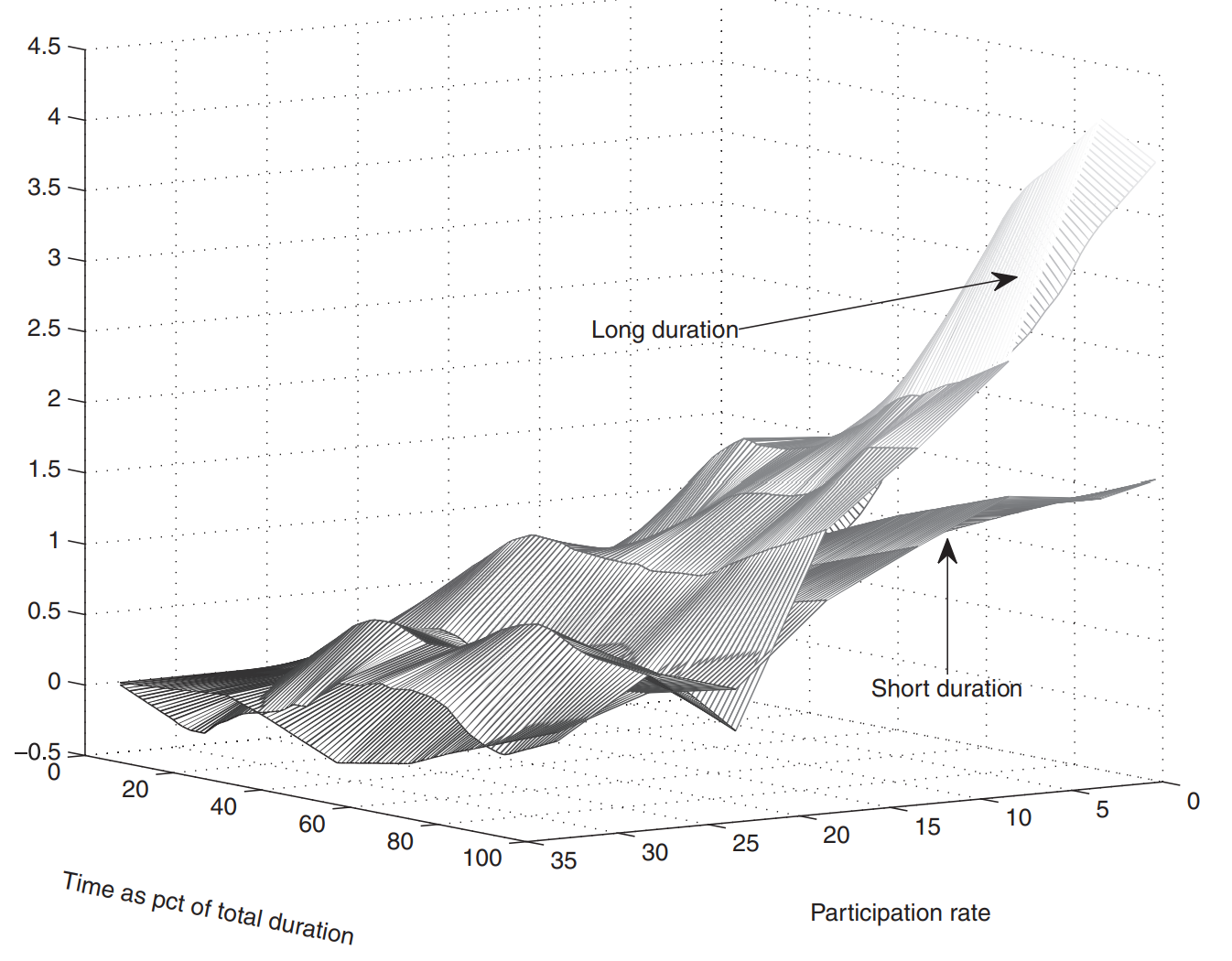
In figure 4 we can see two impact surfaces for two different sets of durations. The surface corresponding to the long duration is always above the shorter duration - ie more market impact. Hence the longer the duration the bigger the impact.

With both participation rate and duration contributing to market impact, we can build the model:

Market Impact

$$\begin{align} \text{Market Impact } \propto \text{Duration}^\alpha \times \text{Participation}^\gamma \end{align}$$

The dependency of the market impact on the two parameters separately is concave. This means the impact of one additional percent of participation rate for an order of a given duration is lower for higher participation vs lower participation.

Market Impact on a Longer Horizon
Within daily data the permanent market impact is the remaining price shift after the decay has taken place. The decay phase starts at the end of the execution period and can not be exactly determined - but we consider that the price reaches its final level after one day. Liquidity providers mostly react at the intraday timescale. After one day the temporary market impact of the metaorder execution vanishes.

Price Anticipation or Permanent Market Impact
There are two positions when it comes to permanent market impact.

Position 1: Permanent impact as the consequence of a mechanical process.

Stock prices move because of the trading of all the market participants. If the selling pressure is stronger than the buying pressure, price goes down and vice versa if buying pressure is the strongest.
We want to understand the law at the root of the impact of buying or selling pressure on price dynamics.

Position 2: Permanent impact as the trace of new information in the price.

Informational vision says stock prices move because new information is made available to market participants. New information allows investors to update expectations which leads to new global equilibriums and price levels.

Permanent Market Impact on a Long-term Horizon

We will look at three studies that de-bias the effect of the signal that triggers price variations. This separates the information effect from the pure execution effect from permanent market impact.

[Bacry et al., 2015]: Reports measures made on a database of electronically traded metaorders from the brokerage arm of a large European investment bank during 2010.

The broker execution database studied does not provide the informational content at the root of the trades.
Authors assumed that the clients of the broker globally constitute a good representative sample of the diversity of market investors (total portfolio not far from CAPM)
The study of price moves on the post-execution period net of market portfolio moves is the so called idiosyncratic moves of stock prices.

[Waelbroeck and Gomes, 2015]: Uses a database of trades from 112 portfolio managers across several large institutional asset managers between 2009 and 2012.

Each trade is labeled as ‘liquidity’ or ‘informed’ trades to separate trades triggered by informational events from the rest.
- Informed: Metaorders coming from portfolio rebalancing.
- Uninformed: Cash trades that are related to new subscriptions of redemptions triggered by heterogeneous and relatively exogenous to the market information.
On a daily basis informed trades have a permanent market impact but uninformed trades do not.

[Brokmann et al., 2015]: Studies a proprietary CFM database consisting of an exhaustive list of 1.6 million metaorders together with the daily signals that lead to these trades over three full years (2011-2013) in a variety of equity markets.

Uses for each trade the signal that triggered it.
Uses the intensity of the trading signal which triggered each metaorder to remove the informational content of their studied proprietary metaorder database.
Divergence of effective and expected price moves gives measure of permanent impact in the absence of informational effect.
Authors observed no permanent impact on the residual price moves.

De-biasing the Temporary Market IMpact of Autocorrelated Execution During th ePOst-Execution Period

All three studies aggregate signed metaorder flows show autocorrelations even several days after execution. This has an effect of post-execution price variations and needs to be filtered out in order to make an accurate estimation of the permanent market impact.

Aggregated daily participation rates are computed at the stock scale as the sum of the signed traded volume divided by the total market volume for the stock on that day.

Total autocorrelations are the equi-weighted average of the autocorrelations across all the stocks of the studied universe.

Finding a unbiased long-term impact picture is not straightforward. Market impact of metaorders according to daily participation rate turns out to be far from linear.

Withdrawing impact of metaorders traded over the post-execution period uses a simple market impact model in [Waelbroeck and Gomes, 2015]. In [Bacry et al., 2015] a square root model is fit. Price variations and the post-execution period are debiased by subtracting the market impact associated to the aggregated daily participation rate on that date applying the square root model.

CAPM Decomposition of Price Variations
[Bacry et al., 2015] uses a CAPM framework to disentangle the systematic component of the market impact form the idiosyncratic components. For each metaorder the decomposition is centered on teh execution dat over a 41-day period:

\[\begin{align} \forall d \in \{D-20, \dots, D, \dots +20\}, \\ \log(P_d) - \log(P_{d-1}) = \beta(\log(I_{d-1})) + \Delta W_d. \end{align}\]

$D$ is the metaorder execution date, $P_d$ is the stock’s close price on date $d$, $beta$ designates the beta of the traded stock on the period from $D-20$ to $D+20$, and $I_d$ is the reference index price on date $d$.

$\beta$ is estimated through simple least mean square regression and the idiosyncratic component starting one day before the execution at date $D-1$ is defined as the cumulative sum of the residuals $\Delta W_d$:

\[\begin{align} W_d - W_{D-1} = \sum^d_{d=D}\Delta W_k \end{align}.\]

The systematic component is defined as $\beta(\log(I_{d-1}) - \log(I_{D-1}))$.

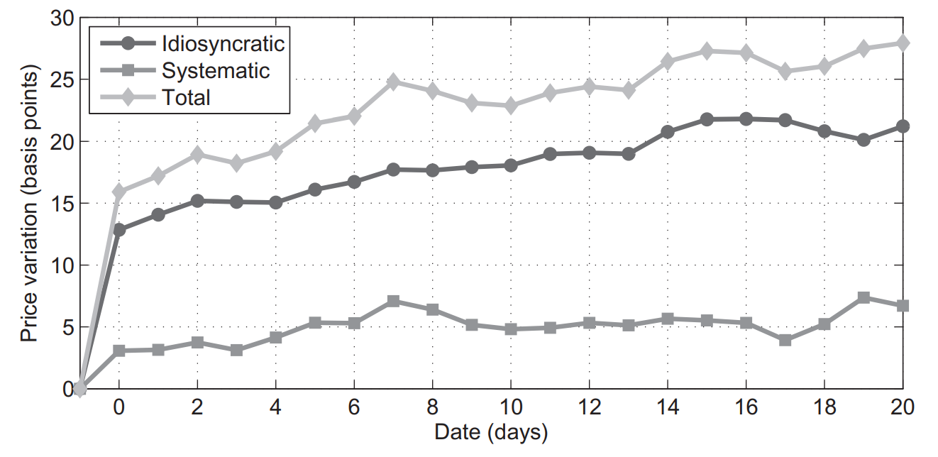
In figure 5 we see the idiosyncratic, systematic, and daily post-execution profiles of price moves. The post-execution profiles of price moves are not yet debiased - the price jump between day 0 and 1 correspond to the market impact of the execution on day 1. Over the time horizon prices slowly trend in the same direction.

After debiasing the post-execution profile the market impact of metaorders executed the day after the execution has been removed. We can see the effect in figure 6.

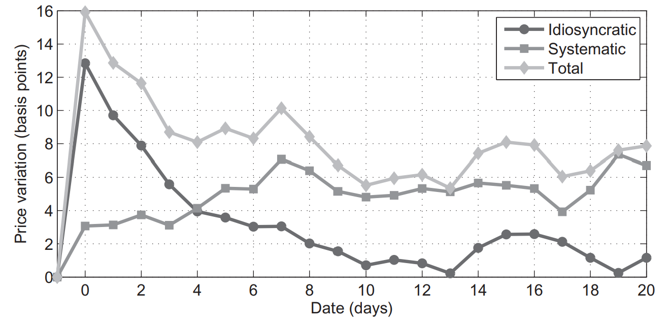
idio_debiased — Figure 6. Post-execution profile without the impact of other metaorders. Price moves are considered relatively to close price the day before execution. Idiosyncratic component + systematic component = total component

Over the post-execution period the price converges back to a level lower than the one reached on execution day. The idiosyncratic post-execution profile reaches its initial level before the end of the observed period - this permanent market impact that remains 20 days after the execution is entirely explained by the systematic component (average level of the market).

Based on this, [Bacry et al., 2015] concludes that once temporary market impact of the correlated metaorders executed has been removed and aggregated information (systematic) has been isolated and removed there is no permanent market impact due to the metaorder itself.

The PFP and Orderbooks Dynamics

On equity markets most trading takes place on LOB that are often called CLOB. This is opposite of a quote driven system (used on fixed income markets).

Attractiveness of Limit Orderbooks
Limit orderbooks are convenient for several reasons:

They are anonymous and provide MLT, leveling the playing field between traders and market-makers.
They are fast and synchronized, easily supporting fragmentation and competition between trading platforms.

By understanding orderbook dynamics one can answer the question: How can practitioners extract information form orderbook dynamics?

Information Reaching Orderbooks
At the start of the day an orderbook is empty. Traders and market makers send orders that are stored in the orderbook if they do not match resting orders - orders are matched if they are compatible in price. Each match generates a transaction and gives birth to three messages:

Public trade
Two private trades: one for each party of the trade

Because the orderbook is hosted on a server in a data center, the localization of the data center is paramount because it influences latency.

Members of the trading facility are connected to the server ina secured way, often via tow channels: one private (SLE) allowing them to send and receive messages to the server and one public channel (SLC).

On the private connection the trader will send specific order to the matching engine and receive answers and messages concerning his orders.
On the public channel they will see the transactions and the state of the orderbook.

The Orderbook in Motion
If the fair price of a stock is around $10, the first trader with intentions to buy will buy cheaper and a selling trader will try to sell for more. This message of buying low and selling high can last long as no transaction occurs. It shapes the orderbook and keeps record (limit-by-limit view) of the sum of all orders at each level of price.

To see the trade the order must be fulfilled. At any point in the life cycle of the orderbook a trader can insert, modify, or cancel an order.

The effect of messages can:

Remove liquidity via cancellation or transaction (Market order or limit marketable order).
Add liquidity via an insertion.

Transactions can only occur at the first limits of the LOB.

Understanding via Conditioning
To use conditioning of the orderbook we focus on the probability that a limit order touches the first limit only when its size is large. Is the probability different from the probability of an insert at the second limit when it is small?

This conditioning can be split into three trends:

Zero-intelligence: Has few conditioning and instead focuses on identifying the distribution of variables of interest.
Game theoretic: Explains the behavior of participants with accuracy. Tries to deduce the theoretical laws for probability of each type of order.
Empirical: Authors estimate transitions empirically.

Poisson Modeling
We can use the point process to model the probability of occurrence of an event. Poisson processes are standard point processes with intensity $\lambda$. Let $N$ be the number of occurrences of an event, then we can same for some time $t$:

\[\begin{align} \lambda = \lim_{\Delta t \to 0}\frac{\mathbb{E}(\Delta N)}{\Delta t}. \end{align}\]

If we know $\lambda$ then the average number of events observed during $\Delta T$ can be approximated using $\lambda \times \Delta T$.

Hence we can isolate three intensities in the orderbook:

$\lambda^+$: limit order
$\lambda^c$: cancellation
$\lambda^x$: transaction

Plain Homogenous Poisson Modeling
The simplest model for the three intensities is to use the homogenous Poisson framework. The probability to observe a liquidity consuming or liquidity providing event is independent of the state of the orderbook.

We can estimate the intensities by starting at time $t$ and record the timestamps of the next event in each category, which we denote $\tau^+, \tau^c, \tau^x$. Obtain the observations of time to wait $\tau - t$ then average them out over the whole database for an estimate of $1/\lambda$.

With the three intensities we can simply run a simulation of the random dynamics of an orderbook and look at the distributions of the queue sizes we obtain during the simulation.

The homogenous Poisson process is very far away from reality. It does not take into account the state of the orderbook. Modeling arrival rate of atomic events (insert, trade, cancel) does not succeed in recovering the observed configurations of queue sizes on the same data.

Improving the Model Based on Conditioning
[Huang et al., 2015] shows a good way to improve the modeling by simply conditioning the three intensities by the size of the considered queue. This is called the Queue Reactive Model.

Model I Instead of avenging the time before events to find the intensity, we keep record of one intensity for each queue size:

Start at time $t$.
Record the queue size $Q_t$ at $t$ in a generic unit.
Observe an event (say $c$) at $\tau^c$.
Keep track of $\tau^c - t$ in a register associated to the size of the queue $Q_t^c$ at $t$.

Iterating over a lot of starting times $t$ gives us a collection of $\tau - t$ for each event. We can now average wait times by queue size.

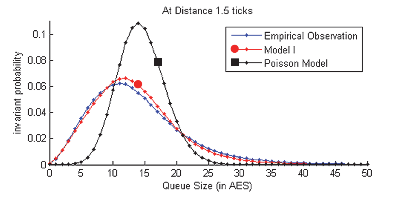
poiss — Figure 7. Asymptotic distribution of the size of the second queue in three cases: Empirical and “Model I” of [Huang et al., 2015] are very close, the Poisson model (upper dark line), is very different. x-axis is observed queue size in AES, y-axis is the probability of occurrence of this size

Model II \& III The distribution of sizes at other limits are not good with Model I, so Model II and III improve the statistics by conditioning intensities by the current size of other queues.

These models condition intensities by the size of the concerned queue but also by the size of its two neighbors. For example the intensity of events ont he first queue should be a function of the current size of the first, the second, adn the opposite first queue. To predict probability $p$ of the number of cancellations int he next 10 seconds on the first bid queue of size 4, we can write:

\[\begin{align} p := \lambda^c(4, 2, 1) \times 10. \end{align}\]

The improvement can be describes by two facts:

When the first queue is smaller than its opposite queue, it will most probably be consumed.
When a first queue is large, the second queue will probably see more cancellations than if the first queue is small.

This is called predictive power of imbalance: liquidity imbalance at the first limit gives a god idea of future price direction.

In most cases the amplitude of this future price movement is lower than a tick size, hence it is not possible to build a rewarding arbitrage on this predictor.

Asymptotic Behaviors of the First Two Queues
A/R ratio (Arrival over Departure ratio): This measures the intensity of insertion over te sum of the intensities of cancellation and trades.

When the ratio is greater thn one,the queue will explode (size will never stop increasing) and when its ratio is lower than one the queue will disappear (size will go to zero).

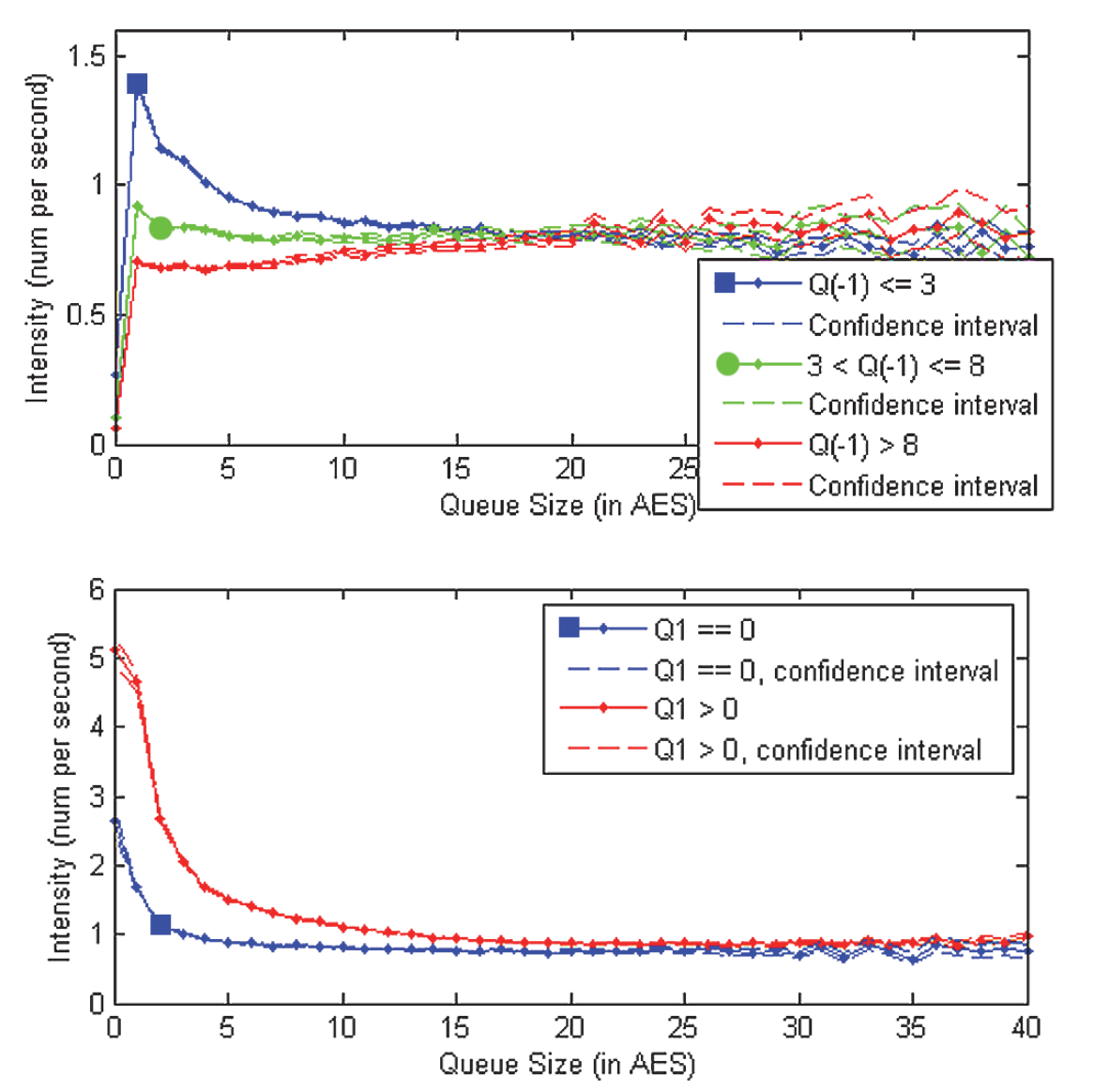
Figure 8. Ratio of incoming over outgoing liquidity on first limit (top) and second limit (bottom) as a function of its size (x-axes)

In figure 8 we can see

The first limit is always depleting to 0.
The second limit explodes.

In the context of stable sizes of the orderbook:

The first queue goes to 0 while the second queue explodes.
Once the first queue disappears the formerly second queue is now promoted as a first queue.
The promoted queue depletes to prevent explosion.

Liquidity Dynamics vs. Price Dynamics

Note an observation: Now that we have a model reproducing with accuracy liquidity dynamics, you can generate realistic orderbook dynamics - but what about price trajectories you generated?

The volatility of these trajectories is far too low compared to the ones observed in the real database used to fit the intensities. This is because in the simulations where a queue is promoted, the sizing of the new first queue is very large. This leads to price reversion - the negative autocorrelation of intraday price returns is a well-known stylized fact, but for an orderbook driven mode, the effect is too strong.

To compensate for the mean reversion we can introduce the following mechanisms:

Time to time: when a first queue fully depletes.
All market participants accept the newly set price as a new ‘fair price: as a consequence the model has to reset the orderbook state to a randomly chosen one in the database.

Summary
The Queue Reactive Model of orderbook dynamics shows the following:

Predictive power of the imbalance of provided liquidity (sizes of first two limits)
The usefulness of the heterogenous Poisson process to roughly model the occurrence of orderbook events.
The need to condition the intensity of the arrival rates of such events byt he size of the concerned queue (and its neighbors).
The need to add a reset of orderbook state after price movement to prevent intense price mean reversion.

When tick size is large the liquidity contained in each queue will be more meaningful than when the tick is small.

The point process in the orderbook is important but other models exist. Instead of counting instance in time, we can count events - changing the meaning of the obtained models. These are called propagator models.

Optimal Trading Methods

Algorithmic trading: Adapting Trading Style to Investor Needs
The following can be noted in electronic execution from investors:

In the US, HFTs are almost everywhere - stealth trading is the main point of focus.
In Asia the comparison between the efficient of trading in each local market is very importance.
In Europe the need to mix between avoiding being detected by HFTs and understanding the efficient of interacting with a set of orderbooks to adjust order routing policies as fast as possible.

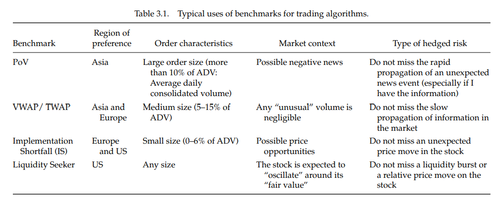
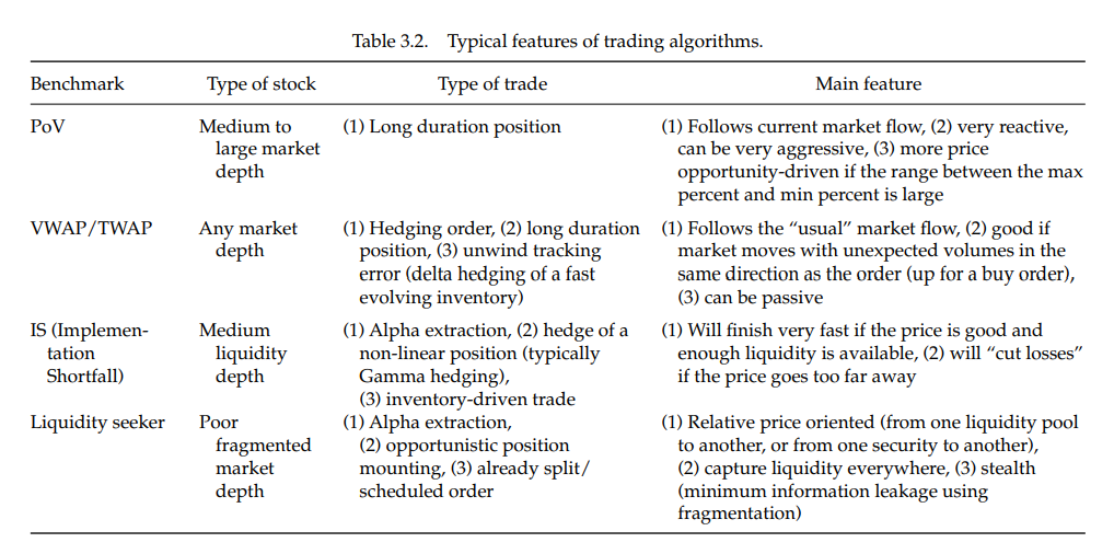
European investors should target Implemented Shortfall benchmarks, Asian ones should focus on VWAP or PoV, and US ones should look at liquidity seekers.

Liquidity seekers are more suitable to trading orders without minimum participation rate constrains, IS are for small orders, VWAP are for larger ones and PoV for very large ones.

The textbook summarizes stock features and features of trading algos in the tables below:

Customization Offers Multi-feature Trading Styles
These benchmarks can be combined: we can add maximum and minimum participation rates to an algo to make it behave like a PoV in the case of a really high or low market volume during the trading.

You can match sophisticated benchmarks like ‘follow market flows if there is high volume, finish fast if the price is really low, and use as much liquidity as possible’ using VWAP or TWAP as a backbone with a minimum participation rate.

Market data needed to build benchmark based policy are noisy because of HFT activity in the orderbook and uncertainty on some important parameters.

From a practical standpoint the optimal trading curve o follow is expressed as a trade rate that has to be represented by the algorithm. If it obtains trades too fast with respect to this curve, it has to stop posting; if it does not obtain enough it needs to obtain trades more aggressively, paying the spread. The curve is not a thin line but a thick one (given noisy data) such that it can define a trading envelope. Inside the envelope any trading trajectory cannot a priori be said to be more efficient than another from a risk-control perspective.

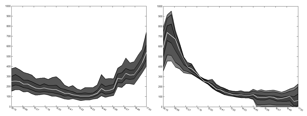
Inside a trading envelope any combination of liquidity capturing techniques can be plugged in without harming the optimality of the risk control layer (strategic layer). It is also possible to inject any volume or price-driven constraints if needed into the way they are built. Customization of a trading algo follows a two step process:

Understanding the desired risk profile and injecting the needed constraints into the trading envelope building process
Understanding the mix of liquidity adapted to the investment style and plugging the associated tactics into the envelopes with respect to properly defined market conditions.

Liquidity Seeking Algorithms are no Longer Nice to Have
Any market participant should be able to evenly access all of the trading venue quoting a given instrument. Any investor should be able to access all the available liquidity at a given marketable price.

In the US the trade-through rule demands that trading venues themselves reroute orders that are marketable at a better price elsewhere. In Europe, the executing broker is in charge of the kind of rerouting - they have to disclose to their clients the best execution policy explaining his rerouting methodology.

The difference is important:

In the US the trading venues have to be able to access an official consolidated orderbook. The clearing and settlement fees/costs have to be the same for all trading venues otherwise a market participant could direct a marketable order on a venue that seems to offer a cheaper price than another (but the participant will pay more, all costs included).
In Europe the executing brokers are in charge to select the way they offer consolidated access to liquidity and have to prove it. It increases the cost of fragmentation for the intermediaries and demands that the investors are able to understand the stakes of these ‘consolidated services’.

Impact of Trading Costs/Fees
Let us denote venue $V$ at price $P$ with fees $f$. Is it cheaper to remove liquidity on another venue $V’$ at a higher price (for a buy order) $P(1+\delta)$, where $P\delta$ is the tick size in euro, because of cheaper fees (say the fees on $V’$ are $f’$ and on $V$ they are $f$ such that $f’ = f - \phi$).

If we have a better price on venue $V’$ than on $V$ we can write: $\begin{align} P(1+\delta)(1+f-\phi)Q <P(1+f)Q. \end{align}$

This is equivalent to having the tick size (in basis points) small enough such that:

\[\begin{align} \delta < (1 - \frac{\psi}{1+f})^{-1} - 1 \approx \phi. \end{align}\]

This means that the tick size should be as small as the fee difference.

A liquidity provider has to be sensitive to the fees he or she will have to pay once this order will be executed. Most times an observer can expect to see limit orders going first on the cheapest venue.

Impact of Latency
It can be said that what is important is not the liquidity that can be seen in the orderbooks but the probability that you will be able to obtain liquidity at a given price level when your order reaches the orderbooks, taking into account the latency discrepancies between venues, the mirrored orders, and hidden liquidity.

Seeking an Optimal Liquidity Capturing Scheme
Dealing with a marketable order (buy market order or buy order with a limit price higher than the best ask price on at least one trading venue) has shown that effects to take into account are as follows:

Probability of hidden liquidity in the orderbooks.
The probability that when the latency to all venues is not the same, HFTs take advantage of information conveyed by market orders reaching one venue to cancel their liquidity providing orders.

Building a Liquidity Seeker
A liquidity seeker has to take care of the following:

Removing liquidity optimally using estimates of the hidden liquidity, mirrored orders, and latency to each venue open to trading.
Posting limit orders optimally to end an order as fast as possible.

Like in dark pools, liquidity in any pool is clustered. Once a trade has occurred, the probability of observing another one increases.

Using fill rates and real liquidity estimates, we can find the optimized allocation of quantity to trade across different trading venues.

Well, this is the end of my mini series! Don’t fret, I have more microstructure posts coming soon; specifically look out for some analysis on the papers mentioned in the textbook.

But anyways, I hope you enjoyed my aggregated notes, both transcribed and hand written, and that you learned something cool.

As a reward for staying till the end, here’s a picture of Linnea’s cat:

Chapter 2: Market Microstructure in Practice

Blog Archive

Archive of all previous blog posts