Chapter 2: Market Microstructure in Practice
In Chapter 2 of Market Microstructure in Practice by Lehalle and Laruelle we explore the nuances of fragmentation by looking at volume curves, the four main variables of liquidity, market share’s effects on spread, and the agenda of HFTs.
I’ve omitted most of the appendix material, historical analysis of European alternative markets, and the Spanish Experiment. For the curious reader more details can be found in Chapter 2.5.
This post is a continuation of Chapter 1, which can be found under ‘Market Microstructure’ on my ‘Blog Posts’ tab. Happy reading!
Below you can find a pdf of the textbook and my notes:
Intraday Market Share to Volume Curves: Stationary Issues
Not all market participants trade for the same reasons. Hence, when liquidity providers create bridges among pools of liquidity, liquidity remains concentrated.
To catch the reference price, primary markets are preferred because they create these reference prices.
Primary markets maintain a monopoly on the flow of another reference price effect called the Exchange Delivery Settlement Price (EDSP). This is the reference price that will be used for the valuation of the derivatives at the expiry.
Inventory Driven Investors Need Fixing Auctions
Equity trading consists of two types of trading sequences:
- Continuous phase: This consists of immediate trade execution where both sides of the orderbook match.
- Fixing Auction phase: this phase includes both opening and closing auctions that are important to fill and clear the orderbook. One can have up to four auctions at once. Some exchanges omit the continuous phase.
Fixing auctions are used for consensual pricing and to unwind orders with huge volume. During witching days fixing turnover is high given that derivative products that expire are taken or closed during these auctions to benefit form same price.
By concentrating more agents, fixing auctions are allowed to form a more consensual price for the whole volume traded. This is very useful if the price is a reference for many valuations (closing prices usually are) and to build orderbooks before the opening of the market.
Fixing auctions also reduce price impact of a trade given high volatility - enhancement of info revealed during the auction stabilizes volatility and increases price stability.
Rules of Call Auctions
Fixing price is determined by four steps - if the price is not clear by the first step the next step is applied. If the last step is not applicable the fixing price can not be determined.
- Maximum Executable Volume: Establish the price at which the highest quantity will be executed.
- Minimum Surplus: Determine price based on the minimum quantity left in the market at the fixing price.
- Market Pressure: If surplus is wholly on the buy side then the highest potential price is the fixing price. Vice versa is true. If surplus is on both sides then the next rule is applied.
- Reference Price: The reference price is the last price traded.
Different methodologies exist for different exchanges.
Theoretical Matching Curves
The composition of participants is different with opening and closing auctions.
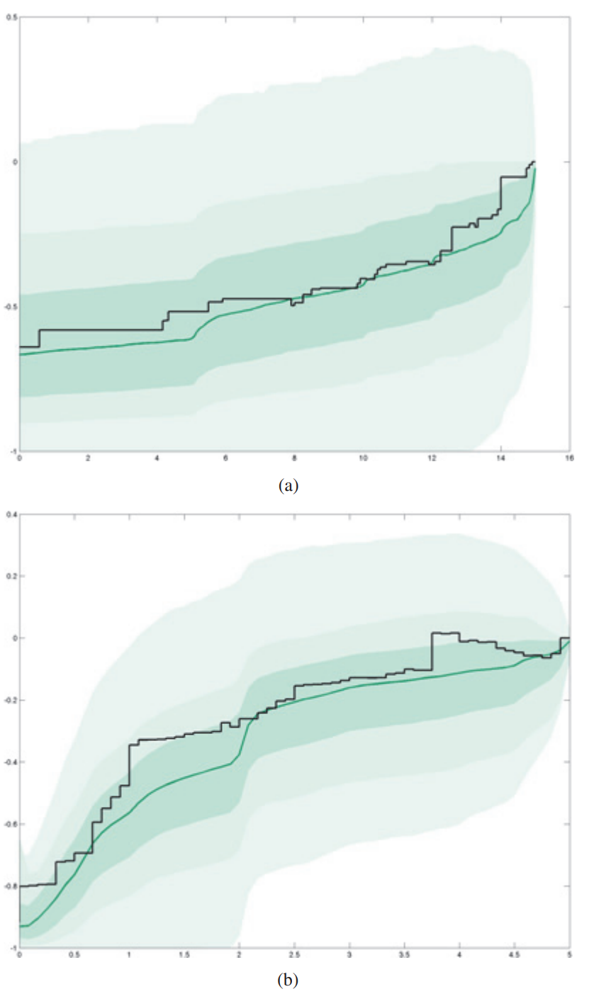
Matching Curves: Relative difference between the volume that would be matched at time $t$ if the auctions ended at time $t$ with the final volume matched at the real fixing for each time $t$.
When a matching curve is zero this means total end volume has been sent to the market - every participant revealed its desire to trade.
In the pre-opening period book building accelerates as time goes on. Matched volume only reaches its final volume in the last few moments. The curve is convex in figure 1.
During closing call, matched volume rapidly increases to its final level as agents already present must participate in the fixing order to close positions. The curve is concave.
Participants take longer to intervene in opening vs closing because there is less uncertainty but also less patience at the end of the day. Participants face most constraints in the closing session given its the last time to open or close a position for the day.
The Opaque German Orderbook
For closing call matching curves in other markets, more than 90% of the distribution remains below the final value. This means that 50% of the time the final volume will be reached before the end of th fixing auction. The upper quartile will go higher than the zero threshold - and given our fixing pricing rules of maximizing volume - this means that a certain amounts of orders needed to be cancelled or modified before the end (around 25%).
In German auctions the orderbook is not revealed. The orders cancelled are probably players fishing for information by cancelling and sending orders to test fill rates. Exploitation/exploration tradeoffs are needed to optimize information levels in the orderbook.
Information Peaks
The pace of information sent into closing and opening auctions follow certain patterns. These updates make matched volume closer to final volume.
Investor Optimal Trading Rate
Market design and information flow timing imply liquidity patterns.
Intraday volume patters allow us to compute execution benchmarks like VWAP and measure how informative traded prices are during intervals. Informed and liquidity traders have in best interest to time their trades together. The meeting of these points create specific intraday volume patterns.
The U and J shapes seen in figure 2 should be analyzed with different causes in context:
- Opening of a linked market.
- Release of news at a predetermined time of day on a regular basis.
- Computation of reference prices and if fixing phase is used for this purpose.
- For many European funds the reference price is the closing price. India does not have a closing price and instead uses VWAP over the last half-hour of trading.
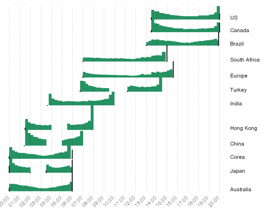
Hong Kong’s volume pattern is shown to be highly dependent with the way reference price is computed.
Brazil’s opening hours are slow until US markets open 30 minutes later. At this time the Brazilian markets will have real price formation; Brazil’s markets are heavily dependent on the US’, instilling winter and summer hours to be more closely matched with US hours. This same market dependency can be said about South African markets and European markets.
Effects of Volume Patterns
Opening of the US Markets:
- NY shift: Computed volume pattern using days where there is only a 5-hour difference between French time and US time.
- Increase in volume occurs when the US markets are open one hour earlier.
- Spikes on the third Friday of March and select months are due to expiry dates.
- NY Closed: Volume pattern on the days where the US market is closed but the French market is open. Activity volume is much lower.
US macroeconomic news:
- Immediate release of economic activity reports on volume depend on how surprising it is for the market.
Equity derivatives expires:
- Witching days and expiry days make investors who do not want to roll over positions unwind cash positions and generate huge volumes during certain time stamps.
- The exchange date settlement price (EDSP) for single stock futures and options is the closing call auction price. This is why closing fixings have large volume as well.
Fragmentation and Evolution of Intraday Volume Patterns
Market share is more important at the beginning vs end of the day. This is because beginning PFP is taking place on the primary market from unmatched opening fixing orders. As well, mature players will time SORs to not route orders to MTFs at time if not needed.
Chi-X’s Jan-Feb 2012 dip (below the 50% threshold) can be explained by the influx of liquidity providers who need to increase activity at the end of the day.
Participants unwinding their cash hedging positions at a price close to EDSP will want to trade on markets where the price will be observed to target reference prices and directly participate in its fixing with their own execution prices.
Four Main Liquidity Variables
The four main liquidity variables are:
- Traded Volume
- Bid-Ask Spread
- Volatility
- Quoted Quantities
Given the state of microstructure and associated trading offers, liquidity providers and consumers explicitly or implicitly accept to trade. The amount traded reflects fragmentation.
Offered liquidity
- Offered liquidity serves as the counter part for traded volume as a variable for liquidity. It can be approximated as the first limit of the books.
Book size, liquidity in the book:
- The book size is the average between the quantity at the best bid and at the best ask. (for smaller tick sizes several limits will need to be summed compared to larger ticks).
- Book size is significant for maximum tradable quantity and serves as a lower bound for traded volume. This concepts is more complex given orderbooks replenish.
All in all book size is an indication of interest of liquidity providers who are ready to trade at the current prices (around mid-price).
The bid-ask spread is the best lowest ask and the highest buy. An instrument is less liquid if the spread is tighter and vice versa.
Comparing bid-ask spread $\psi_1$ vs $\psi_2$ you will find that
\[\begin{align} \psi_i = a + b \cdot \frac{1}{\sqrt{N_i}} \cdot \sigma_i \end{align}\]$N_i$ is the average number of traders per day. $a, b$ are constants that seem to be shared by all instruments given an asset class.
Using $\eta$ we can compute the bid-ask bounce to be,
$$\begin{align} \psi_i = a + \frac{1}{\sqrt{N_i}}(b_1 \cdot \sigma_i + b_2 \cdot \eta \cdot \text{ tick}) \end{align}$$
$\eta$ is estimated using traded price and
- $N^a$ of alternations of price over the day
- $N^c$ of continuations of price over the day
Then,
\[\begin{align} \eta = \frac{N^c}{2N^a} \end{align}\]$\eta$ is influenced by the bid-ask bounces. The more bounces the more alternations and the smaller the parameter. If prices move randomly then $\eta$ is balanced. This parameter can be used to predict the effect of a tick change.
Intraday Seasonalities
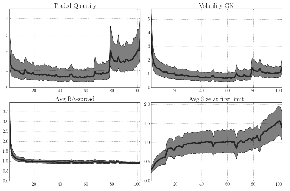
Traded volumes, bid-ask spreads, quantities at first limits, and volatility exhibit intraday patterns. They correspond to more uncertainty on the price after the opening, less activity during mid-day, and a run to end trading before the close. Scheduled events like news influence these patterns.
Volatility is estimated by different models such as Brownian models. Implied volatility can be used as a proxy for volatility but this measure looks at uncertainty of future prices. In the context of microstructure we need to understand the frictions of past trading activity.
The naive estimator of volatility is not a good estimator because of pollution of bid-ask bounce.
In figure 3 we see that the four curves exhibit intraday seasonality. Traded volume, bid-ask spread, and volatility are high at the start of the day. By mid day the price formation process readjusts prices and movement has calmed. By the end of the day volume increases given participants trying to close positions.
When bid-ask spread is large the volume on the book is rather small and vice versa. At the end of the day the spread is at its minimum and when it is at its minimum the book size increases to compensate. Liquidity providers who can’t step into the spread (given its size is the tick size) will have to increase sizes at best bid and ask to provide liquidity, hence increasing the book size.
When the spread is stuck to one tick an increase in the book size plays a role similar to a spread decrease.
Does More Liquidity Guarantee a Better Market Share?
Before MiFID, transactions took place on single national exchanges where liquidity providers and investors were mandated to interact in the same place. Now, with the introduction of competition, exchanges have to attract and keep market-makers, transforming investors into connected members.
Market-makers are attracted through maker/taker fees. Members are attracted through connections costs.
The number of connected member and the satisfaction of market makers is conditional on the liquidity of the exchange
Liquid stock: High volume combined with low volatility and bid ask spread.
Creating and maintaining a trading venue requires:
- Liquidity providers
- Competitive bid-ask spreads
- Connected members
Bid-Ask Spread’s Influence on Liquidity
- The higher the volume on a trading venue the more its market share.
- Volatility cannot be considered as an element of market design choices for an exchange.
The bid-ask spread represents the reward given to the market maker for the risk of providing liquidity.
The bid-ask spread is a way for exchanges to grab market share by increasing the chances the venue hosts a transaction. This is different in the US where mandates for best executions are implemented by consolidated tape.
The Bid-Ask Spread and Volatility Move Accordingly
The daily bid-ask spread increases with daily volatility.
The higher the volatility the higher market makers ask to compensate for their possible loses. This can be modeled with a simple linear regression where volatility can be adjusted per trade (seen in figure 4).
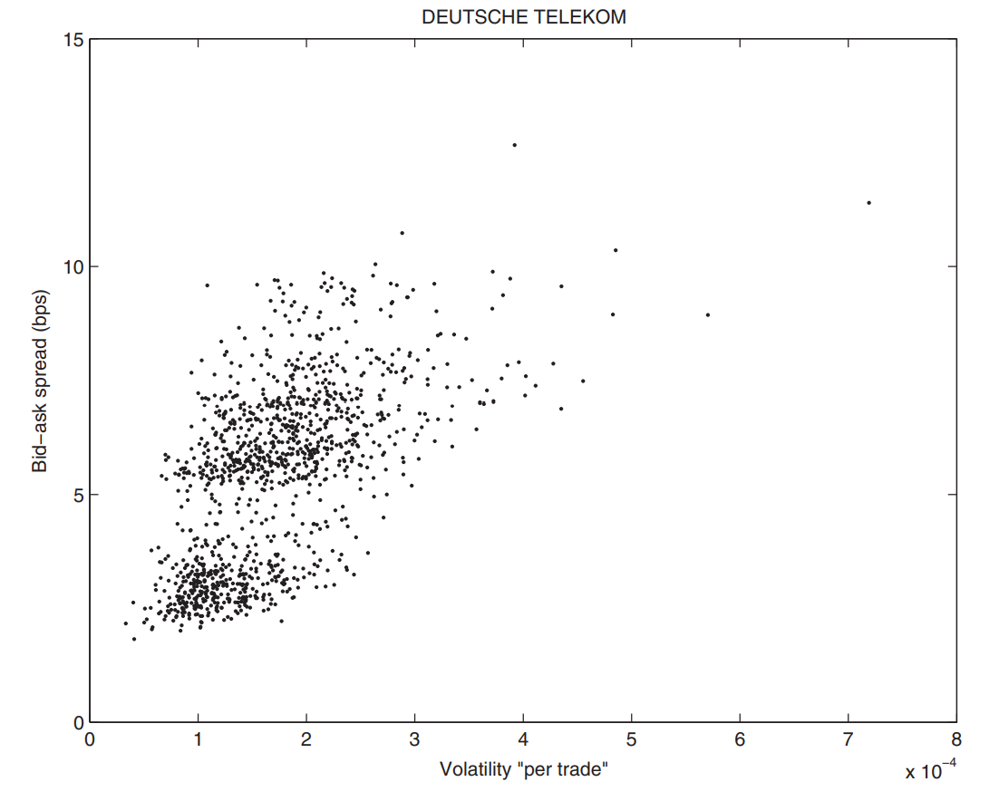
For contributions of microstructure, short term intervals need to be taken into account. After the opening of the market, the market suffers through lots of noise; hence the bid-ask spread and volatility are high. Movement dies down in the middle of the day but picks up by closing because of HFTs needs to flatten residual inventory, making them accept tighter bid-ask spreads regardless of risk.
Bid-Ask Spread and Market Share are Deeply LInked
Market maker activity is more risky on less traded stocks - hence their reward is higher. The market share of a venue moves according to the quality of its bid-ask spread in relative terms.
Tight relative bid-ask spreads imply an increasing market share because SORs are mandated to generate transactions on the venue providing the best price.
Exchanges Need to Show Volatility Resistance
The dependence of the bid-ask spread on volatility is taken into account because it has impact on market makers. Because market makers have the duty to provide liquidity to other participants, they will choose markets that are resilient to relatively high levels of volatility.
Resilience can be measure with the relationship between the number of trades on a trading venue and its price volatility.
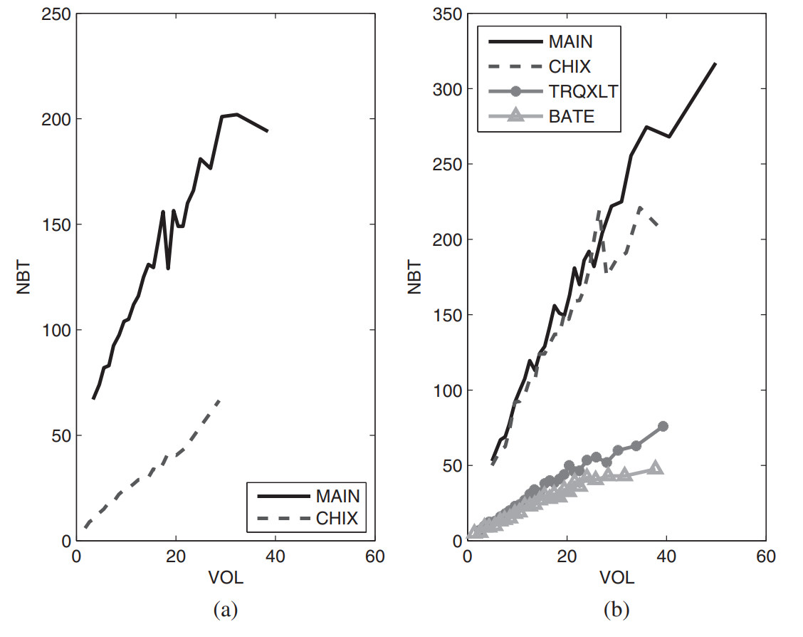
In figure 5(a) the primary market has the highest slope, meaning that it offers a far higher relative number of trades during the volatile periods than other markets. The PFP tends to occur where transactions have the most resilience to volatility, hence Chi-X takes a greater part in the PFP vs. BATS and Turquoise.
But this behavior differs from liquid to illiquid stocks.
Indexes and venues can be compared using the correlation between the number of trades and high frequency volatility. This is called flow reactivity which dictates the hierarchy of destinations. When a venue has low flow reactivity, high frequency market makers stop offering as much liquidity as they do during calmer periods.
There is a strong relationship between quality of trading venue, success, and market makers that operate it. Venues have the obligation to keep market makers active in order to improve market share through competitive spreads and resilience to volatility (better liquidity).
The Agenda of HFTs
The main question concerning HFTs is: Does this market design enable competition between several markets have negative externalities?
Fragmentation was in response to financial market monopolies to decrease prices and increase trading quality.
Metric for the Balance in liquidity Among Indexes Turnover is chosen as a measure of heterogeneity of liquidity among stocks.
We can then ask the question: How well is turnover dispatched between components of indexes? Are only a few stocks responsible for activity on one index or do all components contribute to it equally?
The coverage metric and Gini coefficient evaluate this level of inequity.
Coverage metric:
- This indicates which percentage of the number of stocks is needed to realize 80% of the total turnover.
- This is a static viewpoint that does not take into account the shape of repartition of turnover across stocks. Repartition meaning if the 20% is concentrated over medium traded stocks or spread thinly over low activity ones.
Gini coefficient:
- The Gini coefficient uses the whole repartition curve to estimate the degree of inequality among stocks.
- The repartition curve is found by summing all intraday turnover on each component after the components have been sorted in decreasing order and diving by sum (to normalize).
The Gini index and Kolmogorov–Smirnov test is covered in chapter 1 notes. It can also be reviewed in A.9.
The higher the coverage or the lower the coefficient the more the investor can find an equivalent quantity of liquidity on every stock of the index for a specific exchange.
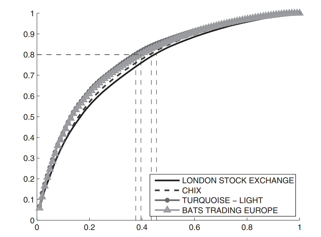
In figure 6 the turnover for 45 FTSE 100 stocks equates to 80% of the total turnover of the entire index on the LSE. By tracing a horizontal line from the y axis where it reads 80% we can find the corresponding x axis value that intersects with the repartition curve. The area under the curve multiplied by two represents the Gini index.
LSE’s coverage liquidity metric is around 45%. The Gini index, which indicates how far the repartition of turnover is from a uniform repartition, is equal to 0.99.
The History of Coverage
Between 2009 - 2012 coverage values increased, decreasing the discrepancies between venues. This created positive homogeneity but did not impact illiquid stocks given HFTs could not increase their activity on them given hedging and short selling is incredibly expensive with large risk.
With the evolution of Multilateral Trading facilities (MTFs), market share became dependent on stock liquidity. Because HFTs have higher risk when extending their activity to less liquid stocks, MTFs increase coverage for wide indexes. Therefore, HFTs extend their perimeter of action for a symbiotic relationship.
High frequency market makers increase uniformity among indexes coverage by spreading volume and ensure the contribution of MTFs to the price formation process by arbitrage.
HFTs Do Not Impact All Investors Equally
Platforms reward trading strategies that make use of the maker/taker schedule. Arbitrageurs use technology to lower inventory risk by trading very small orders very frequently.
The SEC definition for HFTs is as follows:
- Very high speed and sophisticated computer programs for generating, routing, and executing orders.
- Use of co-location services and individual data feeds offered by exchanges and MTFs to minimize network and other types of latencies.
- Very short timeframes for establishing and liquidating positions.
- Submission of numerous orders that are cancelled after submission.
- Ending the trading day in as close to flat position as possible.
How HFTs Lower Spread Without Changing Execution Costs
The effective spread is reduced on an overall basis, but the costs for other participants remain unchanged or slightly increased.
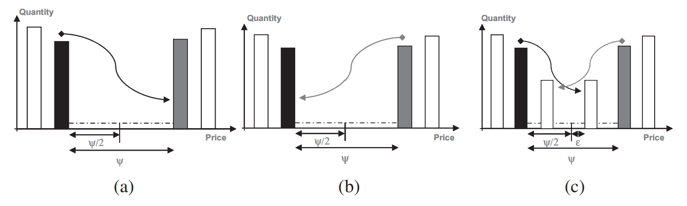
If we consider a market with player A and B, seen in figure 7(a), A becomes impatient and hits player B’s price in order to trade. His cost is the bid-ask spread $\psi$.
In 7(b) player B becomes impatient and hits player A’s price in order to trade. His cost is the bid-ask spread $\psi$. Hence A and B will bear the cost of $\psi / 2$.
In 7(c) a HFT intervenes on the market and takes a position on the outside of B and the first limit against A. A hits the HFT price and his cost is slightly more: $\psi / 2 + \epsilon$. The HFT takes a new position rapidly in front of B, and since B’s order is not matched, B needs to hit the HFTs price. His cost then becomes $\psi / 2 + \epsilon$.
The final effective bid-ask spread is reduced since it represents slightly more than half the formal bid-ask spread. The HFT forces player A and B to become more aggressive, but given trade sizes are small, prompts other participants to fraction their orders, incurring cost. These fixed costs are unevenly distributed and lead to a deterioration in trading conditions for final investors.
Bid-Ask Spread: Cost and Uncertainty for Investors
We now consider if bid-ask spreads would have been unchanged if HFTs had not appeared. If we consider HFTs involved in $q$% of trades, the new bid-ask spread is
The proportion of HFTs among trades is assumed to be 40% and the spreads take the values,
\[\begin{align} \psi_B = 5.41bp\\ \psi_N = 4.73bp \end{align}\]For the cost $C$ the investor has to look at the probability $r$ of meeting a HFT. Three scenarios are outlined:
- If the investor encounters a HFT and is willing to be aggressive the his cost is $C = \psi_{HFT} / 2 + \psi_{B} / 2$.
- If the investor does not encounter a HFT then his cost is $C = \psi_B$.
- If he does not encounter a HFT and is passive he pays $C = 0$.
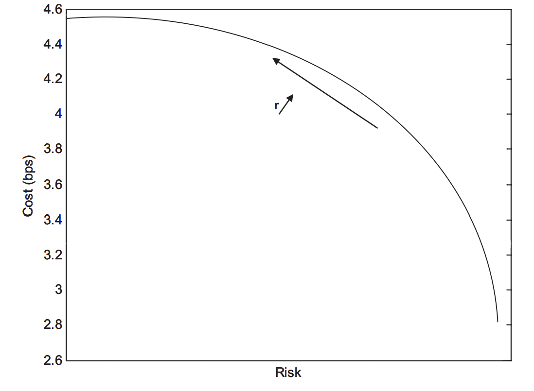
In figure 8 the curve represents $C$ and the uncertainty that relates to $C$. The smaller the cost the higher the uncertainty about it (like the efficient fronter portfolio). Points on the line vary depending on the probability $r$ of meeting an HFT. Increasing this probability increases cost by reduces uncertainty.
For large numbers of trades the Central Limit Theorem (CLT) is used such that,
\[\begin{align} \mathbb{E}[\frac{1}{N}\sum^N_{i=1}C_i] = \mathbb{E}[C] \\ Var(\frac{1}{N}\sum^N_{i=1}C_i) = \frac{Var(C)}{N}. \end{align}\]The uncertainty is lower with the increase of trades.
The bid-ask spread is a source of cost for investors in the market. Both the expected value of this cost and the uncertainty are key figures. Depending on the number of trades and the probability of meeting an HFT actor expectation will not vary but uncertainty will significantly.
The Link Between Fragmentation and Systemic Risk
Systematic risk can be seen as the residual risk that is left in a portfolio when all the other risks have been hedged through all possible financial instruments.
Investors ask if systematic risk has increased with the rise fo HFTs. This gives way to the relationship between extra and intraday volatility. At what extent does extraday volatility effect intraday volatility?
Overnight vs Intraday Correlation
We examine the trends of the average intraday and overnight correlations among the components of an index.
Correlation spikes are often well explained by overnight ones.
Intraday correlation reflects to some extent the amount of co-movement between securities at intraday scale. This is an intermediary marker in the contagion process which leads microscopic causes for macroscopic effects.
To calculate intraday correlation:
\[\begin{align} \text{Intraday Correlation} = \text{Corr(intraday return A, intraday return B), overnight correlation} \\ = \text{Corr(overnight return A, overnight return B)} \end{align}\]where
\[\begin{align} \text{Intraday return} = \log(\text{close}_t)- \log (\text{open}_t) \\ \text{Overnight return} = \log(\text{open}_t)- \log (\text{close}_{t-1}) \end{align}\]During the night the market is organized as an auction fixing and during the day as continuos trading. Hence opening fixing is less liable to be contaminated by loud microstructure noise and tends to reflect consensus of price vs closing fixing. The overnight corrections are closer to extraday correlation.
Flash Crash Analysis
On May 6, 2012 the US stock market suffered a sudden and rapid drop following a rapid recovery.
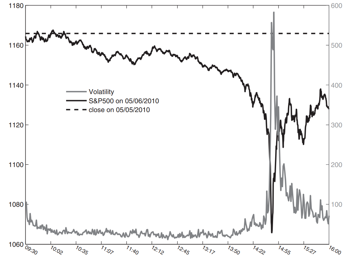
The SEC and CFTC suggested several reasons. The large sale of US indexes on May 6th initiated by a trader who did not put a limit price on the algorithmic order caused an excess of volume that brought HFTs to hedge themselves in light of high risk that day. The snowball effect of hedging eventually returned to its starting point and caused escalations of volume while liquidity offered remained unchanged. The artificially increased volume caused traders to increase flow sent to the market and fed the vicious cycle.
The jump in volume in the market was followed by a large number of HFT players liquidating their positions, increasing imbalance between the demand and supply of liquidly.
The E-mini and SPY showed desynchronization. With the nigh volatility b=on both derivatives, this caused an interruption in the number of orders which transmitted a shock to the stock market. With a pause on orders and the re-routing of OTC orders to primary markets, the pressure on the aggressive side of the orderbook was rising.
As well the Liquidity Replenishment POint (LRP) that slackens the market for a period of time for liquidity to return exacerbated the imbalance between supply and demand. When LRP is triggered all aggressive orders are rerouted to other exchanges - the immediate effect of removing passive liquidity in the NYSE but retaining aggressive liquidity is disastrous.
Systematic Risk and Circuit Breaking
The Flash Crash raised new concerns about the stability of markets. Automation of market making seems to allow liquidity providers to suffer from less adverse selection (because they process information faster). If adverse selection of market makers is a stabilizing force for the PFP, then it can be expected that the more aware adverse selection providers are, the less stable the markets.
Circuit Breakers
Circuit Breakers may be crucial protection against sudden demand of liquidity by market participants. In principle there is a need to stop the PFP in a local or global scale. For a micro scale how can we differentiae between usual liquidity imbalance vs an unusual one that halts trading? Is it even a good idea to halt trading?
Circuit breaks are expected:
- To be activated ini case of liquidity imbalance, but all of them loo at prices. Instead looking at the conjunction of price moves ad poor liquidity can help define more adequate thresholds.
- To be activated in case of abnormal price swings. One should take into account two levels of volatility (daily and intraday variations) using intraday seasonalites.
- Instruments whose prices are indexed on halted tradable assets should be halted when trading on the latter has been halted. This ensures fair trade.
- Highly correlated instrument should be halted to stop propagation of trading impact.
- Synchronization of circuit breakers should be considered and their propagation effect.
Beyond Equity Markets
Trading Futures
Futures are highly electronified. They have no call auction and participants have to agree on liquid hours during which they trade. Futures usually correlate to trading on equities but some studies suggest PFP on futures leads PFP on their components.
Tick sizes of futures are usually larger and cause lots of bid-ask bounce and price reversion. Sizes of first limits of futures are therefore much larger compared to equities.
Future markets are almost not fragmented given post-trading processes would be more complex if fragmented.
Trading Options
The post-trading process on options is more complex than futures. US options markets are fragmented (European ones are note). The current challenge for options markets is to attract market makers given they only post liquidity in limit orderbooks and the buyside consumes liquidity.
Trading Fixed-Income Products
Fixed income products cover a wide variety of instruments: swaps, bonds, foreign exchange credit default swaps, ect. These highly liquid products are traded on electronic platforms close to equites.
Chapter 2 notes are complete!
The penultimate chapter of Market Microstructure in Practice will focus on optimal organizations for optimal trading - specifically targeting trading structure, market impact measurements, and the PFP dynamics on orderbooks.